Quantum Kernels on Synthetic ICU Data: Tracing a Chance-Level Result to the Encoding
A seeded Qiskit benchmark on synthetic ICU data. Every quantum model sat at chance; rescaling the angle encoding lifted the quantum SVMs to 0.70 to 0.80 ROC-AUC, level at best with logistic regression.
TL;DR. I benchmarked five quantum classifiers (three quantum SVMs, a VQC and a QNN) against three classical baselines for in-hospital mortality, in a pipeline built for WiDS 2020 ICU data but run only on its 5,000-row synthetic fallback. Logistic regression is strongest (ROC-AUC 0.817, 95% CI 0.787 to 0.845), and with the pipeline's encoding every quantum model's interval includes 0.5. For the three quantum SVMs the reason is the useful part: z-scores went in as rotation angles, so on average the quantum kernels rated two patients about as similar as two random states. With the input scale chosen on validation data the quantum SVMs reach 0.70 to 0.80, and an RBF SVM tuned the same way (a post-hoc control) reaches 0.810. The rescaling removes an encoding artifact; it does not show a quantum benefit.
I studied physics and mathematics, and quantum kernels looked like the place where that training meets tabular machine learning. A quantum kernel compares two data points by preparing a quantum state for each and measuring their overlap, in a space that grows exponentially with the number of qubits. The hope is that it separates classes a classical kernel cannot.
My July 2026 write-up of this project, and an earlier version of this page, reported a clean null and read it as a statement about scale: at 200 training rows and six qubits, they said, the quantum kernel was already too concentrated to tell patients apart. A later review of the repo showed that reading was wrong, and how it was wrong is the most useful thing the project taught me.
The problem
The WiDS Datathon 2020 dataset holds about 91,000 ICU stays with 186 columns, and about 8% of those patients die in hospital. The pipeline downloads it when Kaggle credentials are present. Without them it generates a schema-matched synthetic fallback: 5,000 rows, 22% positive, about 3% missing values per numeric column. The real data was never run, so every number below comes from the fallback.
Two properties of the fallback shape everything. The label is drawn as sigmoid(severity - 2.7 + noise), where severity is a weighted sum of 13 inputs, linear in all but temperature (which enters as |temp - 37|). So logistic regression is close to the correctly specified model by construction. And the APACHE hospital-death-probability column is generated as sigmoid(severity - 2.5) plus a little noise, so that one column, used as a score with no model at all, reaches ROC-AUC 0.814 [0.784, 0.844] on the test split, next to logistic regression's 0.817. Every model here competes with a column that already carries most of the answer.
The benchmark can therefore answer a narrow question: on a task where a linear model is nearly right, do quantum kernels reach the classical models, and if not, why not.
Why it mattered
A fidelity kernel is an inner product in a Hilbert space, which is physics I already knew. What it measures about patients is a kernel-methods question, and that half decided the result.
How I built it
One trunk, two arms
The pipeline takes 21 curated features: age, BMI, pre-ICU length of stay, APACHE vitals and labs, the three Glasgow Coma Scale components and the APACHE IVa death probability, plus gender, ethnicity, ICU type and elective surgery. Then:
- Impute and encode. Median for numeric columns, mode for categoricals, then one-hot encoding into 29 inputs. This runs on all rows before the split, so the medians include validation and test rows, a small leak the repo documents.
- Split. Stratified 70/10/20: 3,500 training, 500 validation and 1,000 test rows (22.2% positive).
- Scale. A
StandardScalerfit on the training rows only. - Select (quantum arm only).
SelectKBestwith the ANOVA F-statistic keeps six features, one per qubit: age, heart rate, mean arterial pressure, BUN, the GCS verbal score and the APACHE probability. - Subsample (quantum arm only). Class-balanced 200-row training and test subsamples, 100 positive in each, because the pipeline's quantum kernel runs one circuit per kernel entry, O(N²) circuits in all.
The quantum models take the z-scores from step 3 directly as rotation angles. On the quantum training rows they run from -2.85 to 3.18. For the three quantum SVMs, that detail explains the chance-level result.
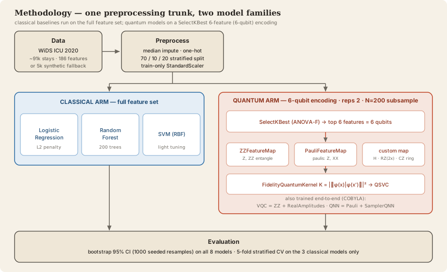
The benchmark pipeline. Both arms share one trunk but see different rows and inputs: all 29 inputs and the full split for the classical models, six z-scores, used as rotation angles with no rescaling, on class-balanced 200-row subsamples for the quantum ones.
Quantum kernels, in plain English
In plain English. A support vector machine classifies a new patient by comparing them with the training patients through a similarity function called a kernel. An RBF kernel calls two patients similar when their feature vectors are close. A quantum kernel turns each patient into a quantum state, using their feature values as rotation angles in a small circuit, and scores similarity as the overlap of the two states: 1 when the states are identical, 0 when they are orthogonal. The SVM never sees the circuit, only the table of overlaps.
In symbols, K(x, x') = |⟨φ(x)|φ(x')⟩|², where |φ(x)⟩ is the state the feature map prepares from patient x. The repo builds it with qiskit-machine-learning:
from qiskit.circuit.library import ZZFeatureMap
from qiskit_machine_learning.kernels import FidelityQuantumKernel
from qiskit_machine_learning.algorithms import QSVC

feature_map = ZZFeatureMap(feature_dimension=6, reps=2)   # 6 qubits, one feature each
kernel = FidelityQuantumKernel(feature_map=feature_map)    # ComputeUncompute fidelity
qsvc = QSVC(quantum_kernel=kernel)
qsvc.fit(X_train_q, y_train_q)    # X_train_q: (200, 6) z-scores, used as angles as-is
y_pred = qsvc.predict(X_test_q)   # X_test_q: (200, 6), scored against a (200, 200) kernel
The kernel values are exact: FidelityQuantumKernel defaults to Qiskit's reference Sampler, which returns the exact probability of the all-zeros outcome of the ComputeUncompute circuit. Everything runs on a noiseless simulator; there is no hardware in this project.
Three feature maps, which were briefly two
The feature map is the circuit that turns a patient into a state. The benchmark compares three, each with 2 repetitions on 6 qubits:
- ZZ (
ZZFeatureMap, Havlíček et al. 2019): a Hadamard layer,RZ(2φ(x))rotations, then ZZ entanglers that couple pairs of features. - Pauli Z+XX (
PauliFeatureMapwithpaulis=["Z", "XX"]): single-qubit Z terms plus X-basis entanglement. - Custom: Hadamards, then
RZ(2x)on each qubit, then CZ gates in a linear chain on neighbouring qubits. CZ is a fixed Clifford gate, so the data enters only through the single-qubit rotations.
The Pauli map started as paulis=["Z", "ZZ"], which is exactly ZZFeatureMap, so for a while two of the three QSVMs produced identical kernels and identical metrics. The fix switched to XX and added a regression test, test_zz_and_pauli_feature_maps_differ, so the duplicate cannot come back quietly.
Two trainable circuits
The VQC puts a ZZFeatureMap in front of a RealAmplitudes(6, reps=2) ansatz with 18 trainable weights. The QNN uses the Pauli Z+XX map with 1 repetition and the same ansatz inside a SamplerQNN. Both train on cross-entropy with COBYLA for 60 loss evaluations. Both use Qiskit's StatevectorSampler, which draws 1,024 seeded shots per circuit, so unlike the QSVMs they carry sampling noise.
Classical baselines and error bars
The baselines are scikit-learn defaults with random_state=42: LogisticRegression(max_iter=1000) with its default L2 penalty, a 100-tree random forest, and SVC(kernel="rbf", probability=True). None is tuned. They train on all 29 inputs and are scored on the 1,000 test rows.
Every model gets a 95% percentile interval from 1,000 seeded bootstrap resamples of its test predictions. The classical models also get stratified 5-fold cross-validation within the training split; the quantum models do not.
What the benchmark showed
| Model | Rows (train / test) | ROC-AUC [95% CI] | Balanced acc. |
|---|---|---|---|
| Logistic regression | 3,500 / 1,000 | 0.817 [0.787, 0.845] | 0.651 |
| Random forest | 3,500 / 1,000 | 0.792 [0.758, 0.824] | 0.646 |
| SVM (RBF) | 3,500 / 1,000 | 0.759 [0.721, 0.796] | 0.631 |
| QSVM, Pauli Z+XX | 200 / 200 | 0.522 [0.440, 0.600] | 0.520 |
| QSVM, ZZ | 200 / 200 | 0.513 [0.434, 0.590] | 0.535 |
| QSVM, custom (H, RZ, CZ chain) | 200 / 200 | 0.513 [0.437, 0.591] | 0.490 |
| QNN (SamplerQNN) | 200 / 200 | 0.484 [0.399, 0.559] | 0.505 |
| VQC | 200 / 200 | 0.437 [0.353, 0.518] | 0.450 |
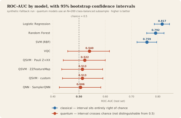
ROC-AUC with 95% bootstrap intervals, synthetic-fallback run. At the pipeline's unscaled encoding every quantum interval includes 0.5.
Every classical interval clears 0.5, and logistic regression's 5-fold cross-validation mean (0.810, standard deviation 0.013) sits on its single-split estimate: stable across folds, on data built for a logistic model. Every quantum interval includes 0.5, and the three QSVMs land within about 0.01 of each other.
The table leaves out accuracy, F1 and PR-AUC because their chance levels differ between the groups: on the 22.2%-positive classical test split, calling everyone a survivor scores about 0.78 accuracy and a random score gets a PR-AUC of about 0.22, while on the 50/50 quantum rows both are 0.5. That is why the quantum F1 values (0.47 to 0.55) look better than the classical ones (0.42 to 0.46). An earlier version of this page blamed over-prediction of the minority class, but a 50/50 test set has none.
Why the quantum kernels sat at chance
The number that gave it away
An audit of the committed results found the kernels concentrated. The ablation below records the mean off-diagonal entry of each 200 × 200 training kernel at the pipeline's encoding: 0.0163 for ZZ, 0.0160 for Pauli Z+XX, 0.0194 for the custom map. Two random 6-qubit states have an expected fidelity of 1/2⁶ = 0.0156. On average, the kernels rated a pair of patients about as similar as two random states.
An SVM's score for a test patient is a weighted sum of K(x_i, x) over the training patients, so it ranks well only if K is large for patients who are clinically alike. With exact kernel values a low average is not fatal by itself; what matters is whether the variation left in K tracks clinical similarity. For the custom map, the one-qubit calculation below shows why that fails at the pipeline's encoding.
A one-qubit calculation
Take the smallest piece of the custom map: one qubit, one repetition, a Hadamard then RZ(2x).
|φ(x)⟩        = ( e^(-ix)|0⟩ + e^(ix)|1⟩ ) / √2           # H, then RZ(2x)
⟨φ(x)|φ(x')⟩  = ( e^(i(x-x')) + e^(-i(x-x')) ) / 2  =  cos(x - x')
K(x, x')      = cos²(x - x')                              # periodic in x - x', period π
Two things follow.
First, the kernel is periodic, and the full custom map is too: RZ(2x + 2π) = -RZ(2x), and fidelity ignores an overall sign. A patient π ≈ 3.1 standard deviations away on one feature, and identical on the rest, gets K = 1, a perfect match. On the training rows the z-scores span -2.85 to 3.18, about two periods, so the kernel's nearest neighbours need not be the clinically nearest patients.
Periodicity also sets the average. Two patients' z-scores on one feature differ with a standard deviation of √2 ≈ 1.4, which spreads their differences across roughly a full period of cos². Averaged over that spread, cos² comes out at 0.509 for independent standard-normal z-scores, almost exactly one half. With six unentangled qubits and uncorrelated features the six factors multiply: 0.509⁶ ≈ 0.017. The real maps add entanglers and a second repetition, so this is only a toy, but the measured means of 0.016 to 0.019 sit where it lands.
Second, the input scale is a knob. Multiply the inputs by s and the kernel becomes cos²(s(x - x')). For small differences, cos²(sΔ) ≈ 1 - s²Δ² ≈ exp(-s²Δ²), the shape of an RBF kernel exp(-γΔ²) with s² in the role of γ. The input scale is a kernel bandwidth, the point Shaydulin and Wild make about quantum kernels. The pipeline had set it to 1 without ever choosing it.
In plain English. A kernel's bandwidth sets how far apart two patients can be before the kernel treats them as unrelated. Too wide and everyone looks the same; too narrow and even near-identical patients look like strangers. Angles add a complication: rotations wrap around. At s = 1 the custom map turns a patient's age qubit two radians for every standard deviation of age, about a third of a turn, so a patient about three standard deviations older comes back to the same state. The kernel's sense of near and far stops matching the clinical one.
The first reading, too few rows, did not survive the ablation below, which keeps the same 200 rows and 6 features and changes only the input scale. The measured mean is consistent with the concentration mechanism Thanasilp et al. analyse, but their subject is how concentration grows with qubit count, which this project never varies.
The bandwidth ablation
scripts/ablate_kernel_bandwidth.py tests the bandwidth reading. It multiplies the six quantum inputs by s from the grid {0.05, 0.1, 0.2, 0.5, 1}, fits the same SVC the QSVC fits on an exact kernel, and picks s per feature map by ROC-AUC on the 500-row validation split, which the pipeline otherwise never uses. Test rows are scored only at s = 1 and at the chosen s, and the script stops unless its s = 1 results reproduce the committed QSVM rows exactly. The sweep and selection rule, from src/qml_healthcare/bandwidth.py without type hints and docstrings:
def sweep_scales(feature_map, X_train, y_train, X_val, y_val, scales):
    rows = []
    for s in scales:                                                        # (0.05, 0.1, 0.2, 0.5, 1.0); 1.0 is the pipeline
        K_train = exact_fidelity_kernel(feature_map, s * X_train)           # (200, 200)
        K_val = exact_fidelity_kernel(feature_map, s * X_val, s * X_train)  # (500, 200)
        _, val_scores = svc_on_kernel(K_train, y_train, K_val)              # SVC(kernel="precomputed"), C = 1.0
        rows.append({"scale": s,
                     "offdiag_mean": offdiag_mean(K_train),
                     "val_roc_auc": float(roc_auc_score(y_val, val_scores))})
    return rows

def select_scale(val_roc_auc):
    return max(val_roc_auc, key=lambda s: (val_roc_auc[s], s))   # best validation ROC-AUC; ties go to the larger s
FidelityQuantumKernel runs one circuit per kernel entry. The exact version simulates each patient once and takes every overlap in one matrix product, so the training and test kernels plus the SVC fit take 0.9 to 5.6 s per feature map, and the whole ablation ran in about 2.5 minutes, on a shared Linux machine. The tests check it against FidelityQuantumKernel to 1e-8:
def exact_fidelity_kernel(feature_map, X_a, X_b=None):
    S_a = _statevectors(feature_map, X_a)            # (n_a, 64): one 2⁶-amplitude statevector per row
    S_b = S_a if X_b is None else _statevectors(feature_map, X_b)
    return np.abs(S_a.conj() @ S_b.T) ** 2           # (n_a, n_b) fidelities
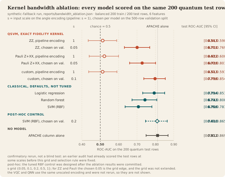
Kernel bandwidth ablation on the same 200 quantum rows. With the input scale s picked on validation data, the QSVMs move from chance to between 0.701 and 0.798. This is a confirmatory rerun, not a blind test.
At the chosen scales the mean off-diagonal entry is 0.24 (ZZ), 0.36 (Pauli Z+XX) and 0.78 (custom), up from 0.016 to 0.019 at s = 1, and every QSVM clears chance: 0.701 [0.631, 0.769], 0.728 [0.660, 0.801] and 0.798 [0.737, 0.854]. Same 200 rows, same 6 features, so the small sample and feature count do not explain the null, though nothing here shows that more rows would make no difference. The best QSVM, custom at s = 0.1, is level with logistic regression refit on these rows at defaults (0.794 [0.731, 0.851]). Neighbouring intervals overlap, so the ablation does not rank the three maps, and no model's point estimate beats the APACHE column alone (0.812), one of the six encoded features.
A fairer control
The comparison still had a tilt: each QSVM had its input scale chosen on validation data, while the classical controls ran at defaults. A later review pointed out the asymmetry, and a post-hoc control, scripts/posthoc_tuned_rbf_control.py, gives the RBF SVM the same treatment: gamma set to scikit-learn's default times s² over the same grid, C = 1, the same selection rule on the same validation rows, test rows scored once. It picks s = 0.2 and reaches 0.810 [0.747, 0.865], a higher point estimate than every QSVM, though the intervals overlap.
At each map's chosen scale, the off-diagonal entries of its training kernel correlate with the tuned RBF kernel's at 0.93 for the custom map, 0.85 for Pauli Z+XX and 0.52 for ZZ. The best QSVM's kernel, once rescaled, tracks a classical RBF kernel closely. The repo's conclusion: "The rescaling removes an encoding artifact; it does not show a quantum benefit."
Three qualifiers belong next to those numbers:
- It is a confirmatory rerun, not a blind test. The audit that found the concentration had already scored the test rows at s in {1, 0.5, 0.25, 0.1}, custom 0.798 at s = 0.1 among them, before this grid and rule were committed.
- Two choices sit at the edge of the grid. ZZ and Pauli both chose s = 0.05, the smallest value tried, and ZZ's validation score was still climbing there (0.505 at s = 1, 0.739 at s = 0.05). The grid was not extended after seeing the results.
- The VQC and QNN were not rerun. They share the unscaled encoding but are also barely trained (below), and neither fix was tested.
What else went wrong
A seed that was not set
The pipeline was described as fully seeded, and the classical and QSVM rows do rerun identically. The VQC and QNN did not: their initial weights and their 1,024-shot sampling both drew unseeded randomness, so reruns of the same code gave different rows. Once both were seeded, the committed VQC moved from 0.540 to 0.437 and the QNN from 0.506 to 0.484. An earlier version of this page listed the VQC at 0.540, the highest quantum row.
The bootstrap interval cannot show a shift like the VQC's (about 0.10), because it resamples test rows only and never varies the seed or the optimizer. Neither circuit is well trained either. With 18 weights and 60 COBYLA evaluations they end at a loss of about 0.955 bits (VQC) and 0.950 bits (QNN), read from the loss curves, barely below the 1.0 bit a constant 0.5 prediction costs. Their chance-level rows say little about what the circuits could learn.
Claims that drifted from the code
An earlier version of this page said the classical models "train 100x to 10,000x faster". The repo revised that to 30x to 30,000x and then dropped any ratio, because it divided quantum times on 200 rows and 6 features, partly from a slower machine, by classical times on 3,500 rows and 29 inputs. It now gives only the ranges, about 37 to 174 s against 0.006 to 1.1 s, and puts the gap on the implementation: with the exact kernel above, the same QSVM fits take seconds, measured on a different, slower machine.
Smaller drifts (a CZ "ring" where the code builds a linear chain, a 200-tree forest where the code has 100, "light tuning" on an RBF SVM that runs at defaults) changed no number. Each changed what a reader would believe about the experiment.
What this does not show
Every number comes from the synthetic fallback; the real WiDS data was never run. No run tests a rescaled encoding or a larger optimization budget for the VQC and QNN, or any change in qubit count, and nothing here has been validated for clinical use. Liu, Arunachalam and Temme (2021) construct a learning problem with a provable quantum-kernel speedup; ICU mortality on tabular features is not known to be one, and nothing here tests that regime. For this task on this data, the repo's verdict is that classical models are the right tool.
Reproducing it
pip install -e ".[dev]"
python scripts/reproduce_all.py              # main pipeline: data, baselines, QSVMs, VQC and QNN, reports
python scripts/ablate_kernel_bandwidth.py    # kernel bandwidth ablation
python scripts/posthoc_tuned_rbf_control.py  # post-hoc RBF control; run after the ablation
The first command needs no account and rebuilds the main pipeline only; a full run took about an hour on a shared 4-core Linux machine, almost all of it in the QSVM stage. The other two rebuild the ablation and its post-hoc control, in that order. Seed 42 sets every split, fit, sampler and bootstrap, and 57 deterministic tests run in CI on Python 3.10, 3.11 and 3.12.
The documentation site has the full method, findings and limitations. Its live demo is a classical logistic regression on six raw inputs, fit on the synthetic data and run in the browser. One input is the APACHE IVa risk score, so, in the repo's words, the demo "scores well for reasons that have nothing to do with quantum computing". It is not quantum and not a clinical tool.
What I took from it
A null result is a claim, and it needs the same checks as a win. "Every quantum model at chance" was true. The explanation attached to it, that 200 rows and a six-qubit circuit had already left the kernel concentrated, was plausible, came with a citation, and was wrong. One number would have caught it early: the mean off-diagonal kernel entry against 1/2ⁿ. I would now run that check before training any fidelity kernel, along with the one-qubit version of the feature map to see what its angles are measured in.
The same thing happened at smaller scale in QML-Essentials. Its week 20 kernel benchmark first read a 4-qubit accuracy drop as kernel concentration, until a post-hoc control that scaled the inputs by 0.1 closed nearly all of the gap to the RBF kernel; the notes now call it a bandwidth effect. In both projects the input scale was a hyperparameter the preprocessing had set and nothing had tuned.
Any knob tuned on one side of a comparison has to be tuned on the other. Against the RBF SVM at defaults (0.708), the best rescaled QSVM (0.798) looked like a quantum kernel beating a classical one. Tuned the same way, in a post-hoc control, the RBF SVM reached 0.810, a higher point estimate than all three QSVMs, though the intervals overlap. The best QSVM is still level with logistic regression on those rows; what the ablation does not show is a quantum benefit.
Provenance decides what a number can claim: which run produced it, which seed, which machine, which rows, and whether the test set had already been seen. Most of the corrections on this page are provenance corrections.
The physics I brought was enough to build the circuits. It did not give me the reflex to ask what the angles were measured in. That reflex comes from kernel methods, and this project is where I picked it up.
The code, results files and full history are at github.com/TirtheshJani/QML-Healthcare-Diagnostics, and the companion post tells the same story more briefly. I had AI coding assistance (Claude Code) on the implementation.