QML-Essentials: a quantum machine learning curriculum, with classical baselines where they apply
Twenty-seven PennyLane and Qiskit scripts, one per curriculum week and all run on simulators, from a Bell pair to a quantum autoencoder. The tier 2 ledger holds no clear quantum win in its seven rows, and the results that taught me the most were the ones that fell apart under a control.
TL;DR. QML-Essentials is a self-study curriculum laid out as 27 weeks, one runnable script each, from circuit basics to a quantum autoencoder, all on simulators. The tier 2 ledger has no clear quantum win in its seven rows; its largest gap, on the kernel task, mostly closes when the inputs are rescaled (a post-hoc control). The 16-parameter autoencoder reaches 0.9871 ± 0.0258 held-out reconstruction fidelity over 5 seeds and ties a 136-parameter classical one, and a post-hoc check shows that an encoder whose code ignores bond length already scores 0.9540 on the same metric.
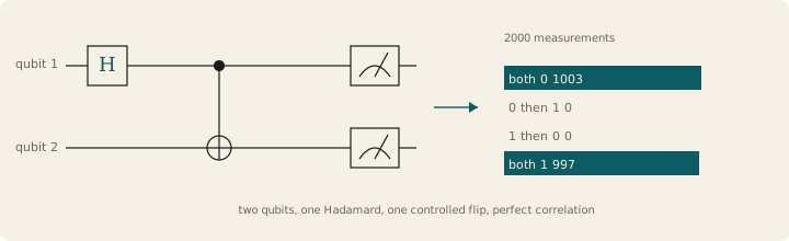
Where it begins. After a Hadamard and a CNOT, two qubits measure 00 or 11, each half the time, and never a mismatch. A coin flip copied onto two bits would do that much. The pair also agrees when both qubits are measured along X (⟨XX⟩ = +1 as well as ⟨ZZ⟩ = +1), and no unentangled pair can do both. That is entanglement, and week 8 checks it.
I came to quantum computing from physics, mathematics and classical machine learning, new to quantum circuits, and QML-Essentials is the side project I used to learn it. The question was narrow: on problems small enough to simulate, does a quantum model beat the obvious classical alternative, or does it only produce a number? So each tier 2 sub-project and the tier 3 autoencoder sit next to a classical reference, and most of what I learned came from rows where that reference, or a simpler control, matched the quantum number.
PennyLane is the main framework because its circuits drop into PyTorch like any other differentiable layer; Qiskit handles a QAOA cross-check (week 14) and the quantum kernel (weeks 18 to 20). Nothing ran on quantum hardware.
The shape of the curriculum
The curriculum runs in three tiers, back to back. Each week is one script plus a notes file.
| Tier | Weeks | What it covers |
|---|---|---|
| I, literacy | 1 to 8 | Bell and GHZ states, teleportation, Deutsch-Jozsa, Grover's search, the quantum Fourier transform, a checkpoint |
| II, core QML | 9 to 21 | VQE, QAOA, a variational classifier, a quantum kernel, a barren-plateau probe, a hybrid capstone |
| III, one artifact | 22 to 27 | A 4-qubit quantum autoencoder on H₂ ground states, with a noise sweep and classical baselines |
From week 8 on, each script ends in assertion gates and exits non-zero if one fails (with one exception, below); weeks 1 to 7 are print-only walkthroughs. CI runs all 27 on pinned requirements. The gates are thresholds committed with the scripts, not pre-registered predictions, and some turned out unable to tell a good model from a trivial one.
Tier I: reading circuits
The first eight weeks had one goal: look at a circuit and predict what comes out. Teleportation (week 3) tests that best. Alice entangles an unknown qubit with her half of a shared Bell pair, measures her two qubits, and sends Bob two classical bits naming the X and Z corrections that recover her state; her copy is destroyed, as the no-cloning theorem requires. Bob's Bloch vector matches her input for six test states to about 5×10⁻¹⁶. Without the corrections he holds, on average, the maximally mixed state, which is why teleportation cannot signal faster than light.
The week 8 checkpoint is set up as a rebuild of Bell-state preparation and Grover's search from first principles, without reusing weeks 2 or 5, and it is the first script with hard assertions. It checks the correlations of all four Bell states (for the pair above, ⟨XX⟩ = +1, ⟨YY⟩ = -1, ⟨ZZ⟩ = +1) to 1e-10. Grover's success probability after k iterations is sin²((2k+1)θ), with sin θ = √(M/N) for M marked items out of N: for one marked item in 16 it predicts about 0.961 at k = 3, and the circuit gives 0.9613.
Tier II: four sub-projects against a classical reference
Each tier 2 sub-project has a classical reference on the same data: an exact solver for 2A and 2B, a trained model for 2C and 2D. Only week 17 is parameter-matched, and most of tier 2 ran at a single seed.
2A. VQE on the hydrogen molecule
H₂ is the one problem in tier 2 that is quantum by nature.
In plain English. A molecule's ground-state energy is the lowest energy its electrons can have. VQE (the variational quantum eigensolver) prepares a trial state with a small circuit, measures its energy, and lets a classical optimizer turn the circuit's angles until the energy stops falling. The variational principle guarantees the result never dips below the true ground-state energy.
In the minimal STO-3G basis, H₂ is a 4-qubit Hamiltonian, and PennyLane's AllSinglesDoubles ansatz gives it 3 angles. Parity forces the two single excitations to zero: each moves one electron from the bonding orbital to the antibonding one, and those have opposite parity, so they cannot mix into the ground state. The double moves both electrons, two parity flips that cancel, and settles near 0.225 rad. At the 0.74 Å equilibrium VQE lands within 0.001 mHa of the exact answer (FCI in this basis, -1.13729 Ha), far inside chemical accuracy (1.6 mHa). Restricted Hartree-Fock is 20.5 mHa too high.
Week 11 reran VQE at 12 bond lengths from 0.40 to 2.50 Å. Hartree-Fock keeps both electrons in one orbital shared by both atoms, but once the bond is pulled apart the true state has one electron on each. The double excitation mixes |1100⟩ with |0011⟩, exactly the freedom needed to follow the bond apart.
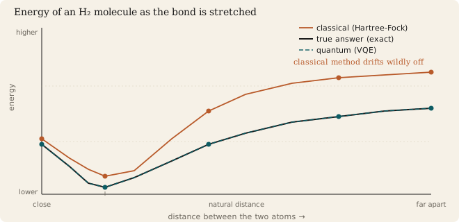
This is the cleanest result in tier 2, and the ledger still scores it a tie: the exact answer came from diagonalizing a 16×16 matrix, trivial at 4 qubits. Behaviour past 4 qubits was not tested.
The week 11 bug
The dissociation script nearly shipped a curve that was pure Hartree-Fock. PennyLane's step_and_cost returns the new parameters together with the cost at the old ones, so a convergence check written the natural way stops at once. The trap, as the week 11 notes describe it:
theta = pnp.zeros(3, requires_grad=True)          # shape (3,): 2 singles + 1 double; zeros = the HF state
e_prev = energy(theta)                            # E(theta_0)
for k in range(max_iters):
    theta, e = opt.step_and_cost(energy, theta)   # returns (theta_1, E(theta_0)), not E(theta_1)
    if abs(e_prev - e) < tol:                     # zero on the first iteration, by construction
        break
    e_prev = e
e_vqe = e                                         # E(theta_0): the Hartree-Fock energy
Zero angles are the Hartree-Fock state, so the loop reports the Hartree-Fock energy at every bond length: a plausible dissociation curve, because it is one, just the wrong one. The assertion at the bottom of the script stopped it, since VQE must sit within 5 mHa of exact everywhere and Hartree-Fock is 20.5 mHa off at equilibrium alone. The committed loop skips the convergence test for the first few iterations and evaluates the energy once more at the final angles. A smooth curve is weak evidence when the wrong answer is also smooth.
2B. QAOA on MaxCut
MaxCut splits a graph's nodes into two groups so that as many edges as possible cross between them. QAOA alternates a layer that phases each assignment of nodes to groups by its cut value with a mixing layer, p times, and a classical optimizer tunes the 2p angles. On a 6-node 3-regular graph, brute force over all 64 assignments (32 distinct splits, since flipping every node gives the same split) finds the optimum of 7 cut edges. QAOA's expected cut reached 0.85 of that at p = 1, 0.94 at p = 2 and 0.98 at p = 3, with 91.6% of the output probability on the six optimal assignments (three splits and their mirror images).
Set beside the Goemans-Williamson guarantee of 0.878, that 0.98 is not a head-to-head: 0.878 is a worst-case bound over all graphs, and brute force solves this instance exactly. A Qiskit re-implementation matched PennyLane to 2.3×10⁻¹⁴ once two conventions were handled: Pauli strings read right to left, and QAOAAnsatz orders β before γ.
Barren plateaus, measured
In plain English. Training a circuit is gradient descent on a landscape. McClean et al. (2018) showed that for sufficiently expressive circuits started from random parameters, the gradient variance shrinks exponentially as qubits are added, until the landscape is flat almost everywhere. That is a barren plateau.
I measured it on one circuit family: RY rotations on every qubit plus a CNOT ladder, stacked as many layers deep as there are qubits. For each qubit count I drew 100 random parameter settings and took the variance of one gradient component, ∂⟨Z₀Z₁⟩/∂θ₀:
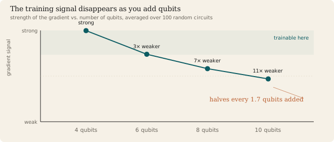
The variance falls 11.4× from 4 to 10 qubits, the steep drop a barren plateau predicts. Four sizes cannot pin down the exponential form (the drop per two added qubits shrinks from 3.3× to 1.7×), so the fitted "halves every 1.7 qubits" is an average over this range, not a rate. The mean gradient magnitude falls less, from 0.246 to 0.075, about 3.3×, close to √11.4: when a zero-centred distribution narrows without changing shape, its typical size tracks the standard deviation. The probe measures a hardware-efficient ansatz, not QAOA, and stops at 10 qubits. It informed the depth of tier 3's encoder: 4 layers on 4 qubits, the probe's n = 4 setting. The repo also cites it for reducing the week 21 capstone's inputs to 4 principal components. Elsewhere the data set the qubit count (four Iris features, 16-amplitude H₂ states), and the kernel has no trainable circuit, so it has no gradients to vanish.
2C. The encoding decides first
The classifier used the harder Iris pair, versicolor versus virginica. Week 15 held everything downstream fixed (4 qubits, an 8-parameter head, 60 epochs) and changed only how the features enter the circuit. On one seed and 20 test examples, angle encoding scored 1.00, IQP 0.75 and amplitude 0.30: 6 of 20, within noise of chance.
The cause sits in the encoder. Amplitude encoding zero-pads the 4 standardized features to 16 amplitudes and divides by the norm, so x, 2x and -x all give the same physical state: length and sign are thrown away. On this pair the classes differ partly in length, so that part of the signal is gone before training starts. It is the general warning in Schuld and Petruccione: the encoding sets a ceiling that no amount of training can lift.
Week 16's hybrid (8 quantum plus 5 classical parameters) scored 1.00 against 0.95 for a single linear layer, one test example from one seed. Week 17 is the repo's only parameter-matched comparison: an MLP with 4 inputs, h hidden units and 1 output has 4h + h + h + 1 = 6h + 1 parameters, so h = 2 matches the hybrid's 13. Comparing the seed-averaged accuracy at each of five training sizes (three seeds each), the MLP won 3, the hybrid 1, with 1 tie (mean 0.943 against 0.923). One test example is 5 points, so the gap is within seed noise.
2D. The largest gap, and what caused it
A quantum kernel uses the circuit only to measure similarity: a ZZ feature map (Havlíček et al. 2019) encodes x as |φ(x)⟩, the kernel is k(x, x′) = |⟨φ(x)|φ(x′)⟩|², and a support vector machine does the rest. The opponent is an RBF kernel, exp(-γ‖x - x′‖²), on Iris setosa versus versicolor, a linearly separable pair. The ZZ inputs were min-max scaled to [0, π], the convention the scripts attribute to Havlíček et al.: each single-qubit angle then spans one period, but the pairwise ZZ angles, built from (π - xᵢ)(π - xⱼ), wind through about three. RBF got standardized inputs. Week 20 swept depth (1 to 3) against training size (20, 40, 80).
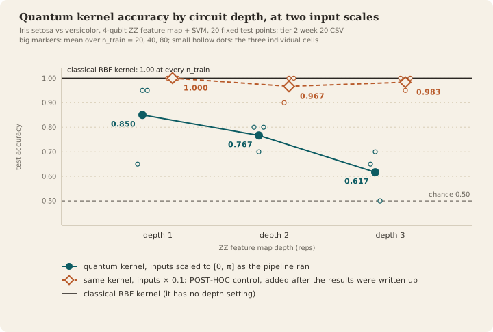
At the input scaling the pipeline used, quantum accuracy falls with depth, from 0.850 to 0.617, and RBF wins all 9 cells. The first version of this page called that the kernel concentration of Thanasilp et al. (2024), seen directly. A post-hoc control, added after those results were written up, says otherwise: multiply the inputs by 0.1 and the quantum kernel scores 0.983 over the 9 cells against RBF's 1.000, with 7 of 9 cells tied and none better.
At 4 qubits the drop is a bandwidth effect. Bandwidth is a kernel's sense of distance: how far apart two points can be before they look unrelated. RBF's default γ is calibrated to standardized inputs; the ZZ map has no γ, so the input scale plays that role, and [0, π] was never tuned as one. At that scale two different training points averaged a similarity of 0.083 to 0.097, near the 0.0625 of two random 4-qubit states; at inputs × 0.1, 0.30 to 0.50. Thanasilp et al.'s concentration grows exponentially with qubit count, which a 4-qubit sweep does not test; Shaydulin and Wild make the bandwidth argument directly.
The × 0.1 factor was the one value tried while reviewing these results, and its effect was known before it went into the script. There was no search over factors, and it is not a gate. Runtime was lopsided either way: 121.1 s for the quantum sweep against 0.099 s for RBF in the committed run. The ratio moves between runs, and it flatters RBF, since RBF's time leaves out building its kernel matrix while the quantum time includes its Gram matrices.
The ledger
| Sub-project | Quantum | Classical reference | Verdict |
|---|---|---|---|
| 2A VQE on H₂ | within 0.001 mHa of exact | exact diagonalization | tie, both exact |
| 2B QAOA, p = 3 | 0.98 of the optimum | brute force over 64 assignments | classical exact |
| 2C hybrid, week 16 | 1.00 | linear layer, 0.95 | +5 points: one test example, one seed |
| 2C matched, week 17 | 0.923 mean | 13-parameter MLP, 0.943 | classical +2 points, within seed noise |
| 2D kernel, week 19 | 0.70 | RBF, 1.00 | classical, at [0, π] inputs |
| 2D sweep, week 20 | 0.74 mean; 0.98 at inputs × 0.1 (post-hoc) | RBF, 1.00 | classical in 9 of 9; post-hoc, 7 ties and no quantum win |
| capstone, week 21 (digits 0 vs 1) | 0.986 | not run | no comparison |
No row is a clear quantum win. The two rows where the quantum method works on a Hamiltonian (H₂ directly, MaxCut written as an Ising cost) are the two where the classical answer is exact and cheap at 4 or 6 qubits; the tabular rows differ by one test example, sit inside seed noise, or, per a post-hoc control, trace mostly to input scale. Schuld (2021) explains why encoding carries so much weight: supervised quantum models are kernel methods, and the encoding fixes the kernel.
Tier III: a quantum autoencoder
In plain English. An autoencoder squeezes data through a bottleneck and rebuilds it. A quantum autoencoder does this to quantum states: a circuit rotates a 4-qubit state so that everything important lands on 2 code qubits and the 2 trash qubits end up in |00⟩. Discard the trash, bring in fresh |00⟩ qubits, run the circuit backwards, and compare with the original.
The data is 22 exact H₂ ground states, bond lengths 0.4 to 2.5 Å, from the 2A chemistry pipeline. An SVD of the 22 × 16 amplitude matrix has two nonzero singular values (4.584 and 0.993): every state is cos t |1100⟩ + sin t |0011⟩, with t moving smoothly with bond length. The data is a 2-D subspace, and one code qubit would have sufficed. That fact explains most of what follows.
The encoder is 4 layers of RY rotations and a CNOT ladder, 16 angles, trained on the trash-fidelity cost of Romero, Olson and Aspuru-Guzik (2017): one minus the mean probability of finding the trash in |00⟩. For a pure input, reconstruction fidelity lies between F² and F, where F is trash fidelity, so the cheap cost brackets the one you care about. The week 23 notes predicted an initial gradient norm near 1.3; the measured 5-seed mean was 0.44, lower than predicted but above the 0.3 gate that checks for a plateau at initialization.
Over 5 seeds (± is the population standard deviation), trash fidelity on all 22 states was 0.9825 ± 0.0214. Trained on 11 bond lengths and tested on the other 11, reconstruction fidelity was 0.9871 ± 0.0258: four seeds at 1.0000, seed 2 at 0.9355. The training states already span the subspace, so the split tests interpolation, not generalization.
What the fidelity gates cannot show
In week 23, seed 2 stopped at a stationary point: trash fidelity 0.9551, gradient norm 0.0000. A check written after all tier 3 results were known (post-hoc, not a gate) explains it.
In plain English. Averaged over all 22 bond lengths, 95.5% of the data lies along a single direction. An encoder that keeps only that direction, and gives every bond length the same code, already scores 0.955. So a score near 0.955 says nothing about whether the encoder learned bond length.
Average the 22 states into one density matrix ρ̄; its two nonzero eigenvalues are λ₁ = 0.955139 and λ₂ = 0.044861. An encoder's mean trash fidelity is Tr(P ρ̄), where P projects onto the inputs it compresses without loss (rank 4 with 2 code qubits), and by Ky Fan's maximum principle that cannot exceed the sum of ρ̄'s four largest eigenvalues. An encoder whose P keeps only the dominant eigenvector v₁ scores exactly λ₁; the part it keeps always lands on the same code state, whatever the bond length:
rho_bar = states.T @ states.conj() / len(states)   # states: shape (22, 16); rho_bar: shape (16, 16)
lam, V = np.linalg.eigh(rho_bar)                   # eigenvalues in ascending order
v1 = V[:, -1]                                      # shape (16,): dominant eigenvector
np.mean(np.abs(states.conj() @ v1) ** 2)           # = <v1|rho_bar|v1> = lambda_1 = 0.955139
The simplest encoder of this kind sends v₂ to that same code state too, with the trash set to 01, so its code is identical for every bond length. That constant code scores 0.9551 on all 22 states and passes every week 23 and week 24 fidelity gate; built from the training half, it scores 0.9540 on test. Seed 2 drops v₂ the same way in both runs: its final loss equals 1 minus the λ₁ of the states it trained on, to six decimals, so its trash fidelity is the constant code's. It sends the discarded v₂ part to a different code state, though, so its reconstruction falls further: the week 24 seed 2 encoder scores 0.9355 on held-out bond lengths, against the constant code's 0.9540.
The bound also caps what any quantum autoencoder can show. A linear projection onto the top 2ᵏ eigenvectors (k code qubits) reaches the same sum, so on compression a quantum autoencoder can at best match PCA. Its case, argued in the repo and not measured, is data access: it acts on the quantum state directly, where a classical model would first need tomography, in general exponentially expensive as qubits are added.
The latent arc that any encoder draws
The first write-up's favourite result was the latent code. The September rerun confirms that PCA on the code qubits' reduced density matrices orders the 22 bond lengths perfectly: Spearman -1.000 for seed 0 (a PCA axis has no preferred sign), in place of the first write-up's +0.998, which no committed script reproduced. It looked as if the encoder had discovered bond length. A control added later showed otherwise. Every state is cos t |1100⟩ + sin t |0011⟩ with t moving monotonically with bond length, so almost any encoder's code features trace a smooth arc that PCA orders by bond length: 999 of 1000 untrained encoders pass the same |Spearman| > 0.9 gate, and the identity gives 1.000. A trained encoder can fail it (seed 2 scores +0.08 in week 23 and +0.24 in week 24), but the gate is applied to seed 0 only. The first version of this page drew the lesson that knowing the physical axis in advance makes a latent space testable; the test also needed an untrained control, and here the untrained control passes too, so passing the gate says nothing about training.
Noise, and the classical autoencoders
Week 25 added a depolarizing channel after every gate (40 in all) and retrained over 3 seeds at each rate; the rates are sweep points, not calibrated to any device. Test trash fidelity fell from 0.971 ± 0.021 at p = 0 to 0.871 ± 0.009 at p = 0.005 and 0.678 ± 0.010 at p = 0.02, heading for 1/4, the value for a fully scrambled trash register. At p = 0.005 that is 61 points above 20 random encoders, but in the post-hoc check the week 24 seed 2 encoder, which keeps only v₁, scores 0.8648 there without retraining, so most of that margin is what any encoder that keeps v₁ gets.
Week 26 gave each state's 32 real numbers (real and imaginary parts) to two classical autoencoders.
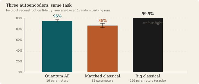
Held-out reconstruction, 5 seeds. The grey diamond is the post-hoc constant-code encoder.
The linear autoencoder (256 weights) is exact, because its 4-number code is larger than the 2-D subspace; here it is an oracle. The small nonlinear one (136 weights) scored 0.9811 ± 0.0211, a tie with the QAE within one standard deviation, where the week 26 notes had predicted about 0.85. Neither is parameter-matched to the QAE's 16, and none could be: a 32 → 1 → 32 autoencoder already has 64 weights.
What went wrong, and what it taught
The first tier 3 review, committed with the scripts, reported 0.946 held-out reconstruction, a Spearman of +0.998, and a "matched" 32-parameter classical autoencoder at 0.86 that the QAE beat by about 9 points. None came from any run of the committed scripts. In September 2026 the scripts were rerun on pinned requirements and every number was replaced with what they print: the "32-parameter" model had 136 parameters, and the 9-point lead became a 0.6-point tie. The first version of this page quoted the old numbers. The week 27 capstone reruns weeks 23 to 26 in one script; it does not check itself against the weekly output, but with seeded runs on pinned requirements its numbers match theirs to the printed 4 decimals.
One gate failed and stayed failed. The first recorded full run stopped at week 23 on its rule that the spread across seeds be under 0.02. The spread was 0.0214, because seed 2 sat at the dominant-eigenvector point and seed 1 was still on a slow plateau when training ended. The threshold was not moved; the script now prints the miss and reports 4 of 5 gates passed.
Other gates turned out weaker than they looked. The Spearman gate passes for untrained encoders, the fidelity gates pass for a code that ignores bond length, and week 23's final-gradient gate passes only because seed 1 is still leaving its plateau. None is pre-registered either: the thresholds have not changed since they were committed, but that commit also held the unreproducible first review, so the history cannot show they were set before the results.
What I took from it
On the question I started with, the answer is the tier 2 review's: on small tabular data with generic features, at simulator scale, classical methods are harder to beat than the marketing suggests. A quantum autoencoder might matter for quantum data too large to read out classically, which the curriculum argues and does not test.
The habit I kept is about controls. Several results here collapsed the same way: a number looked meaningful until something that knew nothing produced it too. Untrained encoders drew the same latent arc, and a constant code passed the fidelity gates. The kernel gap fell to a different trap, a setting (input scale) that one side had tuned and the other had not. The Hartree-Fock curve was a silent bug that the gate against the exact answer caught before it shipped, and the first tier 3 numbers failed on provenance: no committed script produced them. So before I credit a model, I run the same test on the least informed thing that could pass it, I check which setting a comparison left untuned, and I record which script, seed and run produced each number. The stellar spectra audit on this site rests on the same idea, scoring every masked-line effect against random windows.
The repo
The curriculum leans on the free PennyLane Codebook for tier 1 and on Schuld and Petruccione's Machine Learning with Quantum Computers for tier 2. The code is at github.com/TirtheshJani/QML-Essentials-: 27 week scripts with their notes, pinned requirements, CI, and two extra checks beside the tier 3 scripts. The full ledgers and the record of what changed are in TIER2_REVIEW.md and TIER3_REVIEW.md. I had AI coding assistance (Claude Code) on the implementation.