The QSVM Coin Flip Was an Encoding Artifact: Quantum Kernels on Synthetic ICU Data
In July I blamed chance-level quantum SVM scores on the experiment's small size. A later ablation traced them to an unscaled angle encoding: rescaled on the same 200 rows, the QSVMs reach 0.70 to 0.80 ROC-AUC, and a post-hoc RBF SVM tuned the same way scores 0.810, above each on point estimate. All numbers are from synthetic data.
Update, 28 September 2026. I first published this post on 12 July 2026 as "No Better Than a Coin Flip." Its central explanation was wrong; a kernel bandwidth ablation added to the repository in September replaced it, and this version is rewritten around that result. A seeding fix also changed two model rows; that fix and the main other corrections are covered near the end.
In July I had a clean null result and a comfortable explanation for it. I had benchmarked five quantum models against three classical ones for predicting ICU mortality: three quantum support vector classifiers (QSVMs), a variational quantum classifier (VQC) and a quantum neural network (QNN). Every quantum model scored at chance; the classical models cleared it easily. I put that down to scale. At 200 training points and six qubits, I wrote, the quantum kernel "had no room to express structure." It was an easy explanation to accept: it asked nothing more of the experiment and left the door open for quantum methods at a larger size. It was also wrong.
The quantum models still do not win. What changed is the reason, and the reason matters, because a wrong explanation for a null result points the next experiment the wrong way. The July post proposed more training points. For the three quantum SVMs, the real cause came down to one number: how much to shrink the inputs before they become rotation angles. The VQC and QNN share that encoding but were not rerun with it rescaled, and they are under-trained besides.
What was actually run
One caveat governs every number below. The pipeline was built for the WiDS Datathon 2020 ICU dataset (roughly 91,000 stays, 186 columns, about 8 percent mortality), but without Kaggle credentials it generates a 5,000-row synthetic dataset matched to that schema, and every result here comes from the synthetic version. It is 22 percent positive (1,111 of 5,000 rows), and its outcome is a noisy sigmoid of a nearly linear severity score, so logistic regression is close to correctly specified by construction. Nothing here describes real patients, and none of it is validated for clinical use.
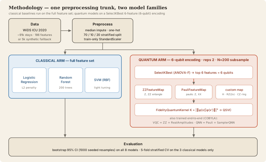
Both arms share one preprocessing trunk but see different data. Median and mode imputation runs on all rows before the stratified 70/10/20 split, so its statistics have seen the test rows; the StandardScaler and the ANOVA feature selection are fit on training rows alone. The classical models (logistic regression, a 100-tree random forest and an RBF SVM, all at default hyperparameters) get all 29 inputs and 3,500 training rows and are scored on the full 1,000-row test split, 22.2 percent positive. The quantum models get the six strongest features by ANOVA F score, one per qubit, on class-balanced 200-row training and test subsamples. Predicting "survives" for everyone therefore scores about 0.78 accuracy on the classical test split and 0.5 on the quantum one, so only ROC-AUC and balanced accuracy share a chance level across the groups. The groups still differ in rows and inputs, which the ablation below controls for.
In plain English. A support vector machine needs one thing from the data: a similarity score for every pair of patients. A quantum kernel computes it with a circuit. Each patient's six numbers set rotation angles on six qubits, and two patients' similarity is how much their quantum states overlap, from 1 for identical states down toward 0. If the overlaps reflect which patients are alike, the SVM can draw a boundary. If every patient looks equally unlike every other, it has nothing to work with.
The three QSVMs differ only in the circuit. The ZZ map is the encoding from Havlíček et al. (2019). The Pauli map uses Z and XX terms on purpose, because Qiskit's ZZFeatureMap is exactly a PauliFeatureMap with Z and ZZ terms; a regression test checks that the two differ. The custom map applies Hadamards, an RZ(2x) rotation per qubit, then a linear chain of CZ gates, a fixed Clifford step, so the data enters only through the rotations. Each map feeds a fidelity kernel computed exactly on a noiseless simulator. The VQC and QNN are trained with COBYLA and sample 1,024 shots per circuit, seeded; the QNN reads out qubit 0.
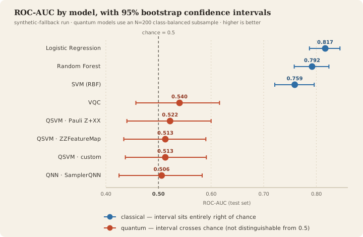
The first result: at the pipeline's encoding, every quantum interval contains 0.5
| Model | Rows (train / test) | Balanced acc. | ROC-AUC [95% CI] |
|---|---|---|---|
| Logistic regression | 3,500 / 1,000 | 0.651 | 0.817 [0.787, 0.845] |
| Random forest | 3,500 / 1,000 | 0.646 | 0.792 [0.758, 0.824] |
| SVM (RBF) | 3,500 / 1,000 | 0.631 | 0.759 [0.721, 0.796] |
| QSVM (Pauli Z+XX) | 200 / 200 | 0.520 | 0.522 [0.440, 0.600] |
| QSVM (ZZ) | 200 / 200 | 0.535 | 0.513 [0.434, 0.590] |
| QSVM (custom) | 200 / 200 | 0.490 | 0.513 [0.437, 0.591] |
| QNN (SamplerQNN) | 200 / 200 | 0.505 | 0.484 [0.399, 0.559] |
| VQC | 200 / 200 | 0.450 | 0.437 [0.353, 0.518] |
At the pipeline's encoding, every classical interval sits above 0.5 and every quantum interval contains it. The brackets come from 1,000 seeded bootstrap resamples of the test predictions, so they cover test-set sampling only, not seeds or optimizer runs.
The classical signal is stable: five-fold cross-validation inside the training split puts logistic regression at 0.810, with a standard deviation of 0.013 across the five folds, right on its single-split estimate. Almost all of it also sits in one column. The generator builds the APACHE hospital-death probability from the same severity score that drives the label, so that column alone, with no model, scores 0.814 [0.784, 0.844] on the same test split, next to logistic regression's 0.817.
Why the July explanation was wrong
July said that at 200 points and six qubits the kernel matrix is close to the identity. The symptom was right: the repository's kernel heatmaps show a bright diagonal on a near-zero field. But a kernel entry is the overlap between two encoded states. It depends on the two patients and the circuit, not on how many other patients are in the training set, so N = 200 cannot make any single entry small.
The encoding can. The pipeline feeds the StandardScaler z-scores, which run from −2.85 to 3.18 on the quantum training rows, straight in as rotation angles, and every map rotates by twice each input: RZ(2x) in the custom map, and a phase of 2x in Qiskit's ZZ and Pauli maps, which also add pairwise phases of 2(π − x)(π − y) for pairs of inputs x and y. What matters is the typical gap between two patients, not the extreme values. A z-score has a standard deviation of one, so two patients' values on a feature typically differ by about one unit; after the doubling, their angles on most qubits differ by a radian or more. Across six qubits and two repetitions of the circuit, differences that large leave two patients about as similar as two random states. The numbers match: the mean off-diagonal entry of the 200 × 200 training kernel is 0.0160 to 0.0194 across the three maps, against 1/64 = 0.0156 for two random 6-qubit states. That is consistent with the concentration mechanism analysed by Thanasilp et al. (2024); how it scales with qubit count was not tested.
In plain English. A classical RBF kernel has a bandwidth: how far apart two points can be and still count as similar. Make it too narrow and every point resembles only itself, so the similarity matrix is all diagonal. Multiplying the inputs by a scale s before encoding does the same job for a quantum kernel; it is the bandwidth studied by Shaydulin and Wild (2022). At s = 1 the pipeline's bandwidth was far too narrow.
The ablation that located the cause
A kernel bandwidth ablation, added after an audit found the concentration, tests this directly. It multiplies the six quantum inputs by s in {0.05, 0.1, 0.2, 0.5, 1}, picks s for each feature map by ROC-AUC on the 500-row validation split (unused by the pipeline), and scores the test rows only at s = 1 and at the chosen s. At s = 1 its exact statevector kernels reproduce the committed QSVM rows, and the main pipeline and its table are unchanged.
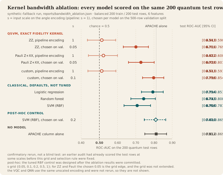
On the same 200 rows and six features, rescaling alone moves every QSVM clear of chance: ZZ from 0.513 to 0.701 [0.631, 0.769] at s = 0.05, Pauli Z+XX from 0.522 to 0.728 [0.660, 0.801] at s = 0.05, and the custom map from 0.513 to 0.798 [0.737, 0.854] at s = 0.1. Nothing else changed, so the sample size and feature count do not explain the null; the encoding does.
Three caveats travel with this. It is a confirmatory rerun, not a blind test: the audit had already scored the test rows at s = 1, 0.5, 0.25 and 0.1, including the custom map's 0.798 at s = 0.1, before the grid and selection rule were committed. The ablation was first labelled pre-specified, and that label was withdrawn. For ZZ and Pauli the chosen s = 0.05 is the edge of the grid, which was not extended afterwards, so a smaller scale might score higher. And the VQC and QNN share the unscaled encoding and were not rerun.
A classical control tuned the same way
A QSVM at 0.798 looks like a rescue until you check what it was compared against. Each QSVM had its input scale tuned on validation data, while the ablation's classical controls ran at default hyperparameters: logistic regression 0.794 [0.731, 0.851], random forest 0.743, RBF SVM 0.708. That asymmetry favours the quantum side. A review pointed it out, and a post-hoc control, designed after the ablation results were committed, addresses it: an RBF SVM with its bandwidth tuned the same way (gamma at its default value times s², C = 1, the same grid, selection rule and validation rows, test rows scored once). It picks s = 0.2 and reaches 0.810 [0.747, 0.865], a higher point estimate than every QSVM, though the intervals overlap.
Two more results point the same way. At each map's selected scale, the off-diagonal entries of its training kernel correlate with those of the tuned RBF kernel at 0.93 for the custom map, 0.85 for Pauli Z+XX and 0.52 for ZZ, so the best QSVM's kernel closely tracks the tuned classical one; ZZ's much less so. And the APACHE column alone, one of the six encoded inputs, scores 0.812 [0.750, 0.869] on these rows, above every model's point estimate, classical or quantum. In the repository's words, the rescaling removes an encoding artifact; it does not show a quantum benefit.
The seed that did not reproduce
The July VQC and QNN rows (0.540 [0.457, 0.616] and 0.506 [0.425, 0.583]) came from a run that was not fully seeded. Neither the initial circuit weights nor the 1,024-shot sampling had a seed, and rerunning the same code gave different numbers (the QNN came back at 0.465). With both seeded, the regenerated rows are VQC 0.437 [0.353, 0.518] and QNN 0.484 [0.399, 0.559], identical on Python 3.11 and 3.12. The VQC's 0.540 had been the best quantum score in the July table; reseeding moved it by about 0.1, and the bootstrap never saw that, because it resamples test rows, not seeds.
Both models are also under-trained: 18 trainable weights, 60 COBYLA loss evaluations, and final training losses of about 0.955 and 0.950 bits (read from the loss curves) against 1.0 bit for predicting 0.5 for everyone. Their rows say little about what these circuits could learn. Neither a bigger budget nor a rescaled encoding was tested.
What else the July text got wrong
- It said all eight models saw the same cohort, split and scoring. They share a split, but not rows, features or test rows.
- It said the split kept an 8 percent positive rate. The synthetic data is 22 percent positive, so an all-negative model scores about 0.78 accuracy on the classical test split, not "in the low 90s."
- It described a 200-tree random forest, a ring of CZ gates with "non-classical" rotations, a parity readout for the QNN and no shot noise. The code uses 100 trees and a linear CZ chain, the QNN reads qubit 0, and the VQC and QNN sample 1,024 shots per circuit; only the QSVM kernels are exact.
- It justified the 200-point subsample by saying the quantum kernel's cost grows with both qubits and training points, and that 200 points already meant 20,000 circuit evaluations per kernel. The 20,000 had no source, and the cost comes from the pipeline's implementation, not from simulating six qubits, as the next point explains.
- It said the quantum models were 100 to 10,000 times slower. That ratio divided 200-row, 6-feature quantum times by 3,500-row, 29-input classical times, so it was not like-for-like, and it is gone. The QSVM fits take minutes because the pipeline's kernel runs one circuit per kernel entry (O(N²) circuits); an exact statevector kernel plus the SVC fit takes 0.9 to 5.6 seconds per feature map, on a different, slower machine.
- It said quantum cross-validation was "not worth the hours." Refits take minutes with the pipeline's kernel and seconds with an exact one; skipping it was a choice.
- It said Liu, Arunachalam and Temme (2021) "identified specific data-encoding regimes" where quantum kernels are provably hard to approximate. They construct a learning problem, built on the discrete logarithm, with a provable quantum-kernel speedup. The same passage put the task at 186 tabular features; the classical models see 29 inputs and the quantum models 6.
- It called feature-map choice noise at this scale. While the kernel is concentrated, the choice cannot show up at all.
- It called the task "real, messy, imbalanced." It was synthetic, and the quantum subsamples were balanced. Its lines about real hardware and a fault-tolerant future had no support and are gone.
Where this leaves quantum kernels
Rescaled, the QSVMs learn this task, so the ablation does not show that quantum kernels cannot. It shows that here, with the encoding fixed, the best of them is level with logistic regression on the same rows, and none beats, on point estimate, a classical kernel given the same tuning or the APACHE column alone. It does not rank the three maps, because neighbouring intervals overlap, and it says nothing about qubit-count scaling, the VQC and QNN at a rescaled encoding, or the real WiDS data, where the gap has not been tested. Liu, Arunachalam and Temme's speedup lives in a constructed problem; ICU mortality on tabular features is not known to be one, and nothing here tests that regime. For ICU mortality prediction on this data, classical models are the right tool.
The July post had an interval on every ROC-AUC and still got its central explanation wrong. An interval covers the sampling noise in a score; the explanation built on that score needs a test of its own. "No room at N = 200" was that explanation, and I never tested it, although July's own text already described the symptom.
What I took from it is a pair of checks to run before reading anything into a quantum kernel score. The first is whether the off-diagonal kernel entries all sit near 1/2ⁿ, judged by their spread in a heatmap and not only by their mean; comparing the mean with 1/2⁶ would already have flagged this pipeline in July. The second is whether the classical baseline got the same tuning budget as the quantum input scale. Without that, a quantum rescue may just be an asymmetry.
Code and reproduction
The repository is MIT licensed and runs offline on the synthetic fallback. One command rebuilds the main pipeline and the eight-model table; the ablation and its post-hoc control need two more, in this order. A full main run took about an hour on a 4-core Linux machine.
pip install -e ".[dev]"
python scripts/reproduce_all.py
python scripts/ablate_kernel_bandwidth.py
python scripts/posthoc_tuned_rbf_control.py
- Code: github.com/TirtheshJani/QML-Healthcare-Diagnostics
- Docs site: tirtheshjani.github.io/QML-Healthcare-Diagnostics. Its demo is a simplified six-input logistic regression, fit on the synthetic data, that runs in the browser: not the benchmark model, not quantum, and one of its inputs is the APACHE-IVa risk score.
I had AI coding assistance (Claude Code) on the implementation.
References
- Havlíček, V. et al. (2019). Supervised learning with quantum-enhanced feature spaces. Nature 567, 209 to 212.
- Liu, Y., Arunachalam, S. and Temme, K. (2021). A rigorous and robust quantum speed-up in supervised machine learning. Nature Physics 17, 1013 to 1017.
- Shaydulin, R. and Wild, S. M. (2022). Importance of kernel bandwidth in quantum machine learning. Physical Review A 106, 042407. arXiv:2111.05451.
- Thanasilp, S., Wang, S., Cerezo, M. and Holmes, Z. (2024). Exponential concentration in quantum kernel methods. Nature Communications 15, 5200.