Decoding the Surface Code: MWPM vs BP+OSD in Simulation
A self-study quantum error correction curriculum whose capstone is a Stim benchmark of two decoders. The fitted thresholds overlap within fit error, the accuracy edge is significant over part of the grid in the committed sweep, and the most useful lessons came from the numbers that later checks took back.
TL;DR. A side-project quantum error correction curriculum whose capstone compares two surface-code decoders in Stim under uniform circuit-level depolarizing noise: minimum-weight perfect matching (PyMatching) and BP+OSD (ldpc). Their fitted thresholds overlap within fit error. BP+OSD makes fewer logical errors at distance 5, significantly so only for p = 0.005 to 0.02 in the committed sweep, on unpaired shots and different error models of the same circuit, at about 600× MWPM's time per shot for sampling plus decoding. Simulation only.
Quantum hardware makes errors far more often than a useful computation can tolerate. Quantum error correction (QEC) is the plan for living with that: spread one logical qubit across many physical ones, keep measuring checks on them, and let a classical program, the decoder, work out what went wrong.
The repo is a curriculum for a reader starting from zero, running from linear algebra to a surface-code decoder study. This page covers what the capstone found and what went wrong on the way: a seed that was not reproducible, a headline number built on a handful of errors, and a textbook code that a notebook first got backwards.
Why the decoder is the bottleneck
You cannot back up a qubit by copying it, and you cannot check it by looking at it, because measurement disturbs it. So QEC measures only parity checks (stabilizers) on small groups of neighbouring qubits. A check reports whether its qubits agree, never what they hold, so the encoded information survives being checked.
A distance-d rotated surface code uses d² data qubits and d² - 1 measure qubits, and repeats its checks every round. Stim, the simulator used here, turns the results into detectors: each compares a check with the same check one round earlier and fires when the two differ, so in a noiseless run no detector fires. A fault lights up a small cluster of detectors, close in space and time. The decoder sees only which ones fired and has to decide whether the logical qubit flipped.
That makes the decoder the bottleneck twice over. Its accuracy sets how much protection a code delivers, and on hardware the detector data never stops arriving, so a decoder has to keep pace as well as be right. The capstone measures accuracy directly, and cost only roughly, as wall time per shot for sampling plus decoding.
In plain English. Picture guards who each watch a few qubits and can only report "these match" or "these don't". Nobody ever says what is being guarded. When something goes wrong, a few guards start shouting. The decoder hears which ones and has to guess what happened, every round, for as long as the computation runs.
Threshold and Λ
Distance d is the smallest number of faults that can flip the logical qubit unnoticed. A distance-d code fails when roughly (d + 1)/2 faults line up badly, so its logical error rate scales like p to the power (d + 1)/2: steeper for bigger codes. At small p, steep is good and the bigger code wins. At large p, the bigger code offers more places for faults and loses. The crossover is the threshold. The repo estimates it by fitting p_L = A · (p / p_th)^((d + 1)/2) to every point at once.
In plain English. Plot logical error rate against physical error rate for distances 3, 5 and 7. Below the threshold the distance-7 curve is lowest: more qubits, fewer logical errors. Above it the order flips. A threshold belongs to a code, a noise model, a decoder and a way of counting errors (per shot or per round). Here the code, the noise model and the counting match. The decoders differ, and so does the form of the error model each one is handed (more on that below). BP+OSD's fit also uses only d = 3 and 5.
Λ is the gain below threshold: Λ(3→5) = p_L(3) / p_L(5), using per-round rates. Λ = 2 means each increase of 2 in distance (3 to 5, 5 to 7) halves the per-round logical error rate. It is the number that turns a target logical error rate into a qubit count.
Where the curriculum stands
| Phase | What it covers | Status |
|---|---|---|
| 0 | Linear algebra, probability, classical error correction | Complete |
| 1 | Qubits, gates, entanglement, density matrices and noise channels | Complete |
| 2 | Repetition code, Shor 9, stabilizer formalism, Steane code, intro to Stim | Partly done: 2.1 and 2.2 in, 2.3 to 2.5 not started |
| 3 | Surface code, MWPM with PyMatching, threshold simulation | Complete, including the benchmark below |
| 4 | Fault-tolerant syndrome extraction, magic states, lattice surgery | Not started |
| 5 | BP+OSD, Union-Find, neural decoders, qLDPC codes | Not started |
The capstone is a first slice: one noise model, two decoders, distances up to 7. The repo's default pytest run has 182 tests, covering the finished phases, Phases 2.1 and 2.2 and the scripts; two slow Monte Carlo tests run separately. Phase 1 overlaps the circuit basics in QML-Essentials.
The benchmark
Circuit, noise and grid
stim.Circuit.generated builds a rotated surface-code memory experiment in the Z basis, run for d rounds. The noise is uniform circuit-level depolarizing: all four of Stim's generated-circuit knobs (after Clifford gates, after reset, before measurement, and on data qubits before each round) equal p. That makes the threshold specific to this model and not comparable to published thresholds under asymmetric models such as SI1000.
MWPM runs at d = 3, 5 and 7 and BP+OSD at d = 3 and 5, over nine p values from 0.002 to 0.025: 27 and 18 cells, seed 42. Each cell draws up to 20,000 shots in batches of 8,192 and stops once it passes 2,000 logical errors. BP+OSD stops at d = 5 because a d = 7 cell takes about 58 ms per shot, too slow for a local CPU.
uv run python scripts/run_threshold_sweep.py \
    --decoder pymatching --noise depolarizing \
    --distances 3 5 7 \
    --p-phys 0.002 0.003 0.005 0.007 0.01 0.013 0.016 0.02 0.025 \
    --shots 20000 --max-errors 2000 --seed 42
Two decoders, two error models
Stim also compiles the noisy circuit into a detector error model (DEM): every fault mechanism, its probability, and which detectors and logical observables it flips.
MWPM treats detectors as nodes and faults as edges, weighted so that likelier faults cost less. It finds the lowest-total-weight set of edges that explains every fired detector (an edge can end on the patch boundary), which is the single most likely explanation, and predicts a logical flip if those edges flip the observable an odd number of times. An edge has only two ends, so every fault must flip at most two detectors, and MWPM gets a DEM decomposed into graphlike pieces. BP+OSD takes the DEM whole. Belief propagation estimates how likely each fault is, and when those estimates do not yield a consistent correction, ordered-statistics decoding solves the parity equations exactly over the most likely faults.
So the decoders do not see the same model. At d = 5 and p = 0.005, 1,101 of the 1,677 fault mechanisms in the undecomposed DEM touch more than two detectors. The comparison below cannot separate the decoding algorithm from the error model each decoder is given.
The code path
The whole pipeline for one point, trimmed from the Phase 3.3 notebook, with shapes added:
import numpy as np

from qec_project.codes.surface import RotatedSurfaceCode
from qec_project.decoders.pymatching_decoder import decode_shots, matching_from_dem
from qec_project.noise.circuit import depolarizing

code = RotatedSurfaceCode.memory(5)        # d = 5, rounds defaults to d
noise = depolarizing(0.005)                # CircuitNoise(p, p, p, p): all four Stim knobs = p
circuit = code.circuit(noise)              # stim.Circuit.generated("surface_code:rotated_memory_z", ...)
dem = code.detector_error_model(noise)     # decompose_errors=True: the graphlike DEM MWPM needs
matching = matching_from_dem(dem)          # 120 detectors, 502 edges

det, obs = circuit.compile_detector_sampler(seed=42).sample(
    50_000, separate_observables=True)
# det: (50000, 120) bool, one column per detector
# obs: (50000, 1) bool, whether the logical observable really flipped
pred = decode_shots(matching, det)         # (50000, 1), the decoder's guess
errors = int(np.count_nonzero(np.any(pred != obs, axis=1)))   # 691 in the committed notebook
A decoder that always predicts no flip makes 11,583 errors on the same shots, so MWPM is 16.8× better than doing nothing. The sweep wraps this loop in harness.sample_cell. BP+OSD enters through a different door:
# harness._compile_decoder: BP+OSD gets the plain DEM, hyperedges included
plain = code.circuit(noise_obj).detector_error_model()

# registry.custom_decoders("bp-osd"): min-sum BP, at most 20 iterations, OSD-CS of order 7
SinterBpOsdDecoder(max_iter=20, bp_method="ms", osd_method="osd_cs", osd_order=7)
ldpc's sinter decoders only implement a file interface, so the harness writes each batch to disk, calls the decoder and reads the predictions back. That interface rebuilds the decoder every batch and decodes shot by shot in Python.
Results
Thresholds overlap within fit error
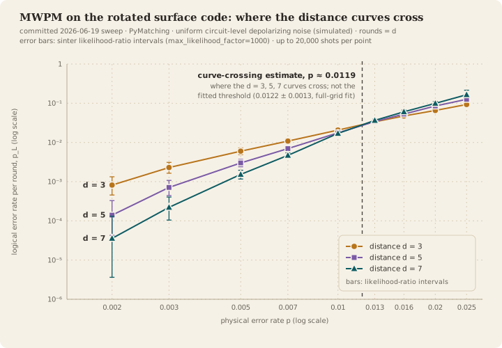
MWPM per-round logical error rate at d = 3, 5 and 7, committed 2026-06-19 sweep (rounds = d). The dashed line is the curve-crossing estimate (p ≈ 0.0119), not the fitted threshold of 0.0122 ± 0.0013. Error bars are sinter likelihood-ratio intervals.
The fit gives p_th = 0.0122 ± 0.0013 per round for MWPM (d = 3, 5, 7) and 0.0134 ± 0.0015 for BP+OSD (d = 3, 5). The difference, 0.0013, is inside the combined standard error of 0.0020, so this data does not rank the decoders by threshold. An early write-up read the gap as a higher threshold for BP+OSD; the error bars do not support that.
The rates are per round. A d = 7 shot runs seven rounds and a d = 3 shot three, so sinter converts each per-shot rate to a per-round one. That puts every distance on the same clock and moves the crossing from near p = 0.007 (per shot) to near 0.012.
The fit window is a systematic: a choice in the analysis, not noise in the sampling, and it can move the answer by more than the error bar. The fit is unweighted over the whole grid, including points well above threshold. A post-hoc fit restricted to p ≤ 0.01 moves MWPM to 0.0101 ± 0.0005 and BP+OSD to 0.0122 ± 0.0013.
The deterministic rerun of 26 September gives full-grid fits of 0.0123 ± 0.0012 and 0.0145 ± 0.0016, a gap of about 1.1 combined standard errors. Both runs put MWPM near 0.012 per round and BP+OSD between 0.013 and 0.015, and neither run separates the two decoders by threshold.
BP+OSD's edge at distance 5
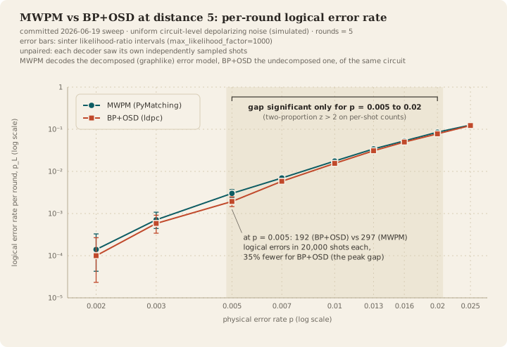
MWPM vs BP+OSD at d = 5, per-round logical error rate, committed 2026-06-19 sweep. The shaded band marks where the gap clears z = 2 on per-shot counts, in this sweep only.
| p | MWPM errors / shots | BP+OSD errors / shots | Gap significant (z > 2) |
|---|---|---|---|
| 0.002 | 14 / 20,000 | 10 / 20,000 | no |
| 0.003 | 71 / 20,000 | 58 / 20,000 | no |
| 0.005 | 297 / 20,000 | 192 / 20,000 | yes |
| 0.007 | 679 / 20,000 | 568 / 20,000 | yes |
| 0.01 | 1,639 / 20,000 | 1,458 / 20,000 | yes |
| 0.013 | 2,442 / 16,384 | 2,238 / 16,384 | yes |
| 0.016 | 3,511 / 16,384 | 3,336 / 16,384 | yes |
| 0.02 | 2,483 / 8,192 | 2,339 / 8,192 | yes |
| 0.025 | 3,136 / 8,192 | 3,093 / 8,192 | no |
In the committed sweep, BP+OSD made 11 to 35% fewer logical errors per shot for p = 0.003 to 0.01, peaking at p = 0.005 (192 against 297). A two-proportion z-test on the per-shot counts puts the gap above z = 2 only for p = 0.005 to 0.02.
Two qualifiers travel with that. The shots were unpaired, so sampling noise sits inside the difference instead of cancelling out. And the range belongs to the committed sweep: the rerun changes which p values clear z = 2.
In plain English. A z-test asks whether the gap between two error counts is bigger than luck usually produces; z above 2 is the usual bar. Unpaired means the two decoders sat different random exams. Giving both the same exam would take a whole source of noise out of the comparison.
Suppression at p = 0.005
At p = 0.005 in the committed sweep, where each cell holds 192 to 355 logical errors, Λ(3→5) is 1.99 (95% interval 1.71 to 2.33) for MWPM and 2.72 (2.27 to 3.25) for BP+OSD, and MWPM's Λ(5→7) is 1.97 (1.65 to 2.35). The intervals come from a seeded parametric bootstrap on the binomial counts, 10,000 replicates. Λ is quoted here and not at the lowest p = 0.002 because those cells hold only 5 to 49 errors; what that did is one of the stories below.
A post-hoc comparison, added after the data was seen, divides BP+OSD's Λ(3→5) by MWPM's. In both runs, the ratio's interval stays above 1 only at p = 0.005; at 0.003, 0.007 and 0.01 it includes 1. At p = 0.005 the committed ratio is 1.36 (95% interval 1.08 to 1.73) and the rerun's is 1.37, but because p = 0.005 is the one p of four where the committed ratio's interval excludes 1, the rerun's 1.37 does not count as a replication of the effect size. That p is also where the d = 5 edge peaks. An effect that shows at one p and not at the three around it is for a paired run, with both decoders on the same syndromes, to settle.
The cost: time per shot
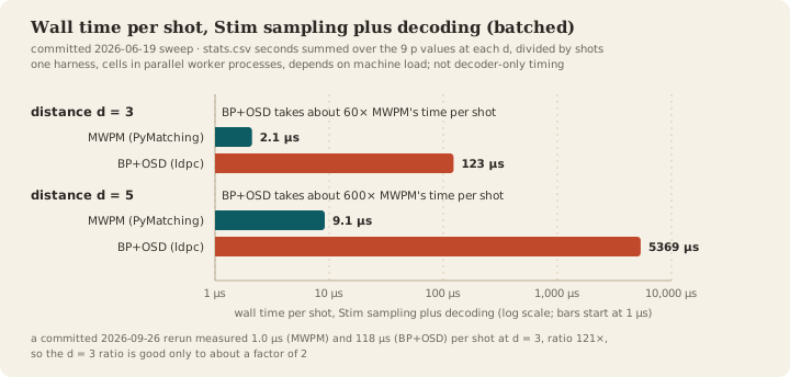
Wall time per shot for Stim sampling plus decoding (batched), committed 2026-06-19 sweep: stats.csv seconds summed over the p grid at each distance, divided by the shots. The 2026-09-26 rerun measured 1.0 µs and 118 µs at d = 3 (121×) and 719× at d = 5.
This is a same-harness comparison, not a decoder-only timing: cells ran in parallel worker processes, so the numbers move with machine load, and BP+OSD's time includes the per-batch rebuild. MWPM's d = 3 time per shot varied about 2× between runs, so that ratio is good only to about a factor of 2. At d = 5 the gap is hundreds of times on this setup, which says nothing about which decoder would keep pace on hardware.
What went wrong, and what it taught
The numbers above survived four rounds of fixes on 26 and 27 September 2026. Most of what changed was how the numbers were read and where they came from; in Phase 2.1, the physics itself changed.
sinter.collect versus NumPy 2
In the locked environment (sinter 1.15, NumPy 2.4), sinter.collect, the usual driver for Stim sweeps, asserts isinstance(errors, int) while np.count_nonzero returns a NumPy integer, so every worker raised AssertionError. Rather than downgrade NumPy, the project wrote an in-process harness that keeps sinter's statistics helpers and the decoder interface BP+OSD plugs into, which meant it now owned its own seeding.
A seed that was not a seed
The per-cell seed mixes the base seed, the distance, p and a salt, a small number derived from the decoder's name. Until 26 September the salt came from Python's hash(decoder), which PYTHONHASHSEED salts per process, so --seed 42 gave different samples in different processes. One cell that holds 355 errors in the committed file gave 345, 342 and 348 under three hash seeds. The fix is one line:
# zlib.crc32, not hash(): str hashes are salted per process (PYTHONHASHSEED),
# which made the seed, and so the samples, change between invocations.
h += (zlib.crc32(decoder.encode()) & 0xFFFF) * 31
That cell now gives 349 under all three hash seeds; Stim guarantees identical samples for the same Stim version on machines with the same SIMD width. A seed only pins a result if everything mixed into it is deterministic too.
Recovering the salts
The committed 19 June files were sampled under unknown salts, and their run.json files name a commit (678ee59) that has no harness, because the sweep ran from uncommitted code. A brute force over all 65,536 values of the 16-bit salt regenerated 37 of the 45 cells exactly (all 27 for MWPM, BP+OSD's 10 at p ≤ 0.01), which ties the files to this harness. The rest is statistical: if the old files came from this harness, a fixed-seed rerun should differ from them only by ordinary sampling luck, and it does (squared differences in standard errors sum to 26.0 over 27 MWPM cells and 15.6 over 18 BP+OSD cells, about the one per cell chance gives). scripts/check_seed_salts.py repeats the exact-match check.
A headline Λ built on a handful of errors
The first write-up, on 19 June, reported Λ(3→5) of 5.8 for MWPM and 6.3 for BP+OSD, taken at p = 0.002, the lowest p both distances share. Those cells hold 5 to 49 errors; BP+OSD's d = 5 cell holds ten. The rerun moved Λ(3→5) at that p to 4.2 and 10.6: one fell by more than a quarter, the other rose by about two thirds. At p = 0.005, with hundreds of errors per cell, it moved from 1.99 and 2.72 to 1.97 and 2.70.
Monte Carlo precision comes from the failures you observe, not the shots you take. Read the error count behind a rate before reading the rate.
A repetition code decided by roundoff
Phase 2.1 simulates the 3-qubit bit-flip code under depolarizing noise, ρ → (1 - p)ρ + p·I/2 on each qubit, averaged over the inputs |0⟩, |1⟩, |+⟩ and |-⟩. Its first version called a trial a failure when the fidelity fell below 0.5, and its write-up described a crossover, the code beating an uncoded qubit at small p. For |+⟩ and |-⟩, every branch with a nonzero syndrome has fidelity exactly 1/2, which evaluates to 0.4999999999999999, so the rule was a floating-point roundoff test. The same rule pinned the uncoded baseline at zero, since a single depolarized qubit keeps fidelity 1 - p/2, which never falls below 0.5. And the committed plot did not come from the committed code.
The fix fails each trial with probability 1 - F, and a test pins the simulation to the exact average infidelity, 0.5·(3q² - 2q³) + 0.25·(1 - (1 - p)³) with q = p/2. The second term carries the lesson. Each qubit takes a phase flip (Z or Y) with probability p/2, which a bit-flip code cannot see, so |+⟩ and |-⟩ fail whenever an odd number of the three qubits take one: about 3p/2, three times an unprotected qubit's p/2. Averaged with the well-protected |0⟩ and |1⟩, that is about 3p/4 against p/2 uncoded. Under depolarizing noise the code is worse than no code at every 0 < p < 1.
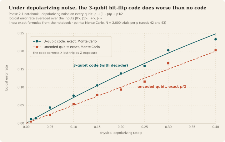
Phase 2.1, corrected: exact formulas from the notebook (lines) and its Monte Carlo run (points, N = 2,000 per p, seeds 42 and 43).
A crossover is exactly the story you expect from an error-correcting code, which is why it needed an exact formula to check against.
Red CI on main
The same Phase 2.1 commit called depolarizing_channel(p), but the Phase 1.3 function of that name takes (rho, p). mypy flagged the call, but the CI mypy step was continue-on-error, so the failure surfaced later as a TypeError in pytest, and CI on main stayed red from 12 July 2026 until the fixes merged on 27 September. The mypy step now blocks. A red build that nobody acts on gates nothing.
"Millions of shots per second"
The Phase 3.3 notebook once said decode_batch "decodes millions of shots per second". Made to time itself, it printed 3.28 µs per shot at d = 5, p = 0.005: about 304,000 shots per second on one core, decode only. The sweep's 9.1 µs per shot at d = 5 includes Stim sampling and parallel workers, which is why every timing on this page says what it includes.
What is next
Phase 2.3 to 2.5, then Phase 4 on fault tolerance. For the capstone: paired decoding, so both decoders see the same sampled syndromes; a control that gives both decoders the same DEM; and a decoder-only timing benchmark. Biased and leakage noise raise NotImplementedError today, because Stim's generated circuits cannot express those channels.
What I took from it
On the decoders: at this scale the threshold fits do not separate MWPM and BP+OSD. Whether a modest accuracy edge at d = 5 is worth hundreds of times the time per shot is a question this setup cannot answer fairly yet: the decoders saw different error models and different shots, and the timing is not a decoder-only cost.
On method, most of what I took away was about what a number is allowed to claim. A salted hash made "seed 42" untrue without anything looking wrong. Low-count cells produced a headline Λ that a rerun overturned. A significance range belonged to one sweep, and a threshold moved with the fit window. Each fix was the same move: record which run produced a number, under which seed and salt, how many failures stand behind it, and which analysis came after looking, then let that decide the sentence. The surface-code physics here is textbook. The provenance I learned by watching it go wrong.
Code, sweep data and figures: github.com/TirtheshJani/QEC-Project (MIT). I had AI coding assistance (Claude Code) on the implementation.