Interventional masked-line ablation reveals partial shortcut learning in a tree-based MK classifier of Gaia-ESO UVES spectra
A LightGBM classifier reaches 0.926 macro-F1 on Gaia-ESO spectra, and an interventional masked-line audit shows one of its three classes is read off non-canonical features instead of the physics.
TL;DR. A LightGBM classifier reaches 0.926 macro-F1 on 3,032 Gaia-ESO UVES spectra across F, G, and K. Two of three pre-specified masked-line ablations land where they should: F collapses without Balmer, G drops 21 points without Mg b. The third does not. K-class accuracy is unchanged at 0.938 when Mg b is masked, and masking Na D or Ca I changes nothing either; K runs on a multi-leg shortcut of Fe I and Cr I lines in the mid-5200 Å region plus the survey pipeline's own continuum level. A Pickles-template cross-check is reported as exploratory, not corroboration. Completed manuscript, May 2026. Zenodo deposit; arXiv submission pending.
A machine learning model trained on stellar spectra reaches a macro-F1 score of 0.926. By every conventional metric, that is a strong classifier. The natural reaction is to ship it, write the paper, and move on.
This paper is about what happens when you do not move on. It asks a different question: when the classifier predicts that a star is type F, G, or K, is it reading the spectral features that an astronomer would use to make the same call, or is it cheating? The answer turned out to be: depends on the class. F and G are textbook. K is not.
The setting in plain terms
Stars are sorted into spectral classes that run roughly hot-to-cool: O, B, A, F, G, K, M. The Sun is type G. The system, called Morgan-Keenan or MK classification, has been the working language of stellar astronomy since the mid-twentieth century. Astronomers identify class by looking at specific absorption lines in a star's spectrum. Hot stars show strong Balmer lines (the hydrogen series including Hα at 6563 Å and Hβ at 4861 Å). Intermediate-temperature stars show the Mg b triplet near 5170 Å. Cooler stars show neutral metal lines like the Na D doublet at 5890 Å and Ca I features at 6162 and 6439 Å. These are the canonical diagnostics, and they are the lines a working spectroscopist would point at.
Modern surveys produce far more spectra than a human can classify by eye. So researchers train classifiers. The question for any such classifier is whether it is doing the job the way an astronomer would, or whether it has found a statistical shortcut, a feature that correlates with class but disconnects from the canonical physics.
Why correlational interpretability is not enough
The standard tools for opening up a model are SHAP, permutation importance, and saliency maps. They rank features by how the model uses them. They do not, however, test whether a feature matters in a falsifiable sense. A feature can rank high because it correlates with a hidden temperature proxy. A feature can rank low because the model has redundant predictors and treats it as substitutable. Neither outcome tells you what would happen if you simply removed the feature and asked the model to classify again.
This study uses an interventional probe: interventional masked-line ablation. For each combination of (diagnostic line, class), the bins covering the line are replaced with a continuum value, the masked spectrum is rescored against the same trained model, and the resulting accuracy drop is compared to a null distribution made from 500 random non-line windows of the same total width. Pre-specified in a version-controlled decision log before the held-out test set was scored (not lodged with an external registry, so "pre-specified," not "pre-registered"). Bonferroni-corrected. Bootstrap confidence intervals. The output is a single number per pair with a p-value, and that number is falsifiable in the strong sense: if it disagrees with the prediction the audit set up, you know the prediction was wrong.
The dataset and the classifier
The audit was run on 3,032 high-resolution spectra from the Gaia-ESO Survey, taken with the FLAMES-UVES spectrograph at the VLT in Chile. The sample distributes as 536 F-class, 1,534 G-class, and 962 K-class stars after quality cuts. The wavelength window covers 4800 to 6800 Å, which contains all the canonical FGK diagnostics.
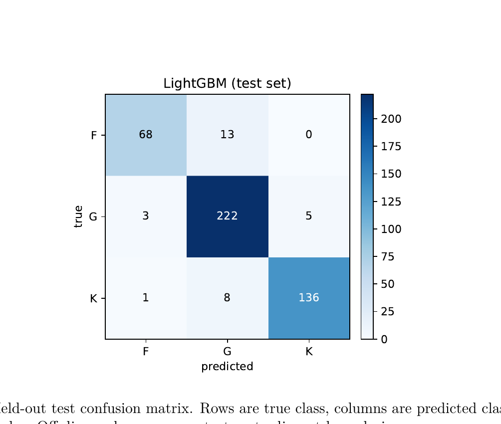
A LightGBM classifier (gradient-boosted decision trees) was trained on the spectra after a fixed train/validation/test split. On the held-out test set of 456 spectra, it scored:
- F-class: precision 0.94, recall 0.840, F1 0.89
- G-class: precision 0.91, recall 0.965, F1 0.94
- K-class: precision 0.96, recall 0.938, F1 0.95
- Macro-F1: 0.926
Recall is quoted to three decimals because per-class recall on the held-out set is, by definition, the same quantity as the per-class baseline accuracy the ablation table below is measured against. Same number, two names.
Held-out test set · 456 spectra
A leakage-aware spatial cross-validation (DBSCAN-grouped K-fold over sky coordinates) returned a macro-F1 of 0.903, against 0.913 for standard stratified K-fold. The 1-percentage-point gap sits in the minimal-leakage band reported by Blanco-Cuaresma (2019). The held-out test score sits 1.5 standard deviations above the spatial-CV mean, comfortably within sampling fluctuation.
So the classifier is real. The next question is how it works.
The audit, one pair at a time
For each (line set, class) pair, the audit measures the accuracy change when the bins covering the line are replaced by a continuum value:

Significance is a permutation p-value against 500 random non-line windows of matched width, using the Phipson-Smyth (B+1) correction so the p-value can never be a misleading zero:

The intervention itself is small. Given the feature bins covering a diagnostic line set, replace them with the continuum fill and re-score the unchanged model (the production code lives in the repo's src/interpret/ module; this is a trimmed, illustrative version):
def masked_accuracy(model, X, y_true, line_bins, fill):
    X_masked = X.copy()
    X_masked[:, line_bins] = fill          # do-operation on the input domain
    y_pred = model.predict(X_masked)
    return (y_pred == y_true).mean()

delta_A = masked_accuracy(model, X_test, y_test, mgb_bins, CONTINUUM_FILL) \
        - baseline_accuracy                # negative delta means the model needed the line
Three headline pairs were pre-specified: Balmer lines on F-class, Mg b on G-class, and Mg b on K-class. The first two are textbook predictions: an astronomer who masked the Balmer series in an F-type spectrum would expect classification to fall apart, and the same for Mg b on G. The third pair (Mg b on K) was the interesting case, because correlational SHAP analysis already hinted that K-class might not be reading Mg b.
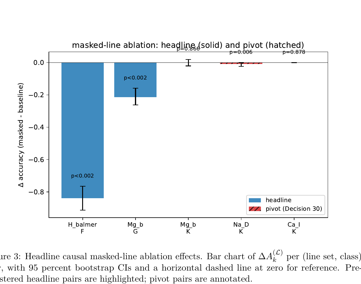
| Line set | Class | Baseline acc. | Masked acc. | Δ | p-value | Verdict |
|---|---|---|---|---|---|---|
| Balmer | F | 0.840 | 0.000 | -0.840 | not reported here | canonical dependence |
| Mg b | G | 0.965 | 0.752 | -0.213 | p < 0.002 | canonical dependence |
| Mg b | K | 0.938 | 0.938 | 0.000, CI straddles zero | 0.866 | no dependence |
| Na D | K | not reported here | not reported here | -0.007, CI includes zero | not reported here | no dependence |
| Ca I | K | not reported here | not reported here | 0.000 | not reported here | no dependence |
The top two rows are what an astronomer would draw on a napkin. Strip the Balmer series out of an F-type spectrum and the class has nothing left to stand on, so every F prediction cascades to G or K, which is exactly the hierarchical Balmer-then-Mg b reasoning a human classifier uses: with Balmer information removed, F spectra read as cooler. Strip Mg b out of G and the class gives up 21 points. The bottom three rows are the surprise. K-class holds its 0.938 recall without measurable functional dependence on three of the canonical neutral-metal diagnostics, and the Mg b p-value of 0.866 says the observed effect is indistinguishable from masking a random stretch of continuum.
What the K-class reads instead
The per-class SHAP traces give the answer.
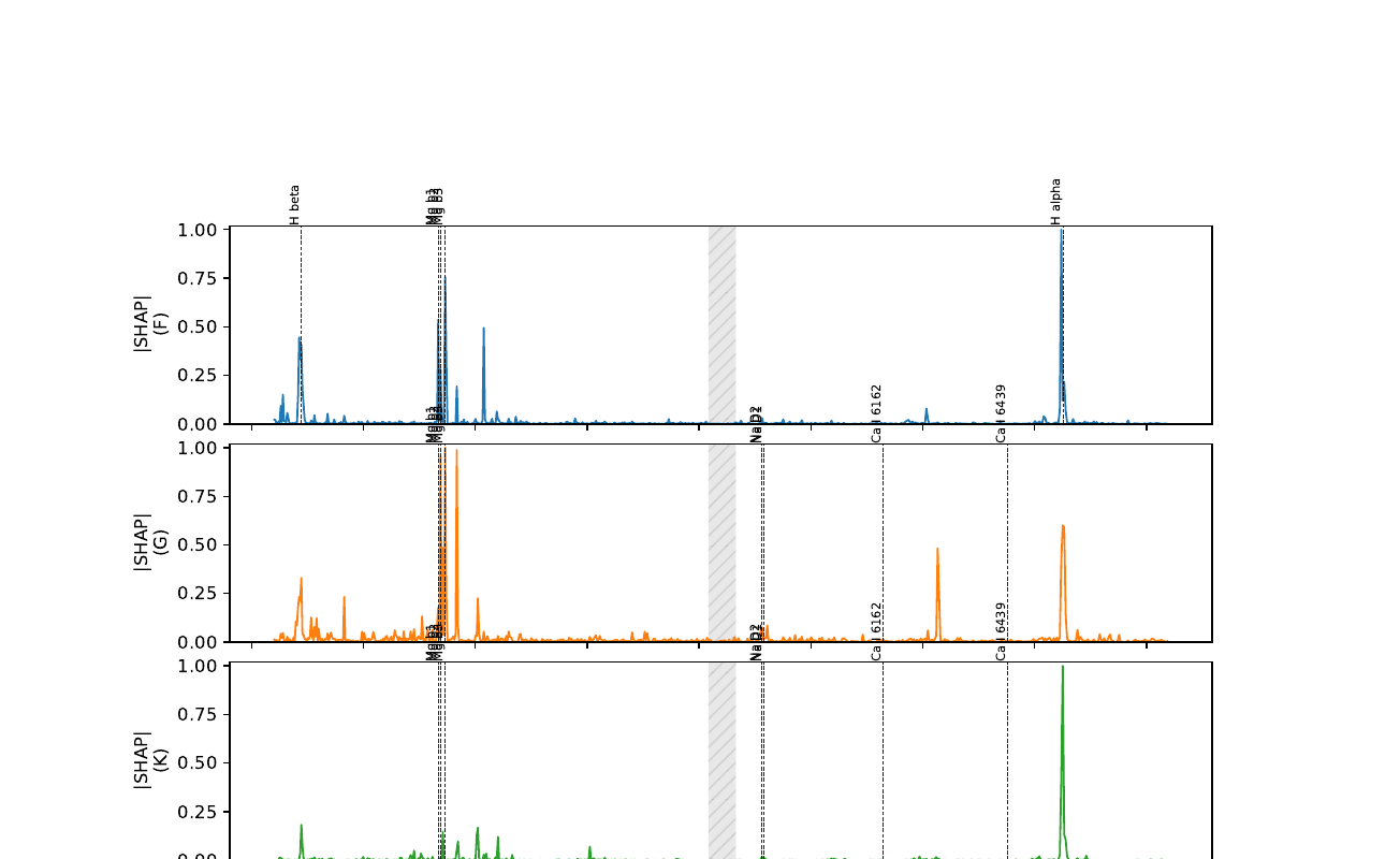
The K-class classifier reads Fe I and Cr I multiplets in the mid-5200 Å region (specifically Fe I at 5269.54 Å and Cr I at 5206, 5208 and 5345 Å) plus the wings of Hβ and Hα. None of these are wrong features for K-class diagnosis. Iron and chromium line strengths track temperature in K dwarfs, and Balmer wing depth, while not a textbook K diagnostic, carries real spectral information that a tree ensemble can monotonize against the F-G-K sequence. The model has learned a temperature-correlated proxy, and the proxy works because at signal-to-noise ratios above 20 over 696 wavelength bins, there are many features that monotonize against temperature. A gradient-boosted tree does not need any one of them in particular.
This is partial shortcut learning. The aggregate metric is fine. The model is internally inconsistent: physics-aware on F and G, proxy-driven on K. Without an interventional audit, the gap is invisible.
The shortcut the SHAP plots could not see
The per-line story is only half of it. The larger finding came from re-deriving the continuum itself. When the inherited Gaia-ESO pipeline normalization is replaced with an independent iteratively sigma-clipped 5th-order Legendre fit on the same held-out rows, and the unchanged model is re-scored, G-class baseline accuracy collapses from 0.965 to 0.148. The dominant misclassification is G to K: 126 of 230 G-class rows reclassify as K.
The model had been using the survey pipeline's per-class continuum level as a non-line G-versus-K discriminator. In the production feature matrix the per-row median flux runs 0.929 for F, 0.919 for G, 0.902 for K, a 2.7-point spread that is monotone with temperature and separable class to class (pairwise KS p at or below 1.6e-3 on adjacent classes). Lift the continuum to a per-class median near 1.0 and that discriminator disappears, so G predictions migrate to the class whose original continuum sat lowest.
None of the correlational tools would surface this. SHAP, permutation importance, and sliding-window occlusion all operate on bin-level attribution inside a fixed normalization. The continuum-level signal is a property of the per-class distribution of an aggregate, the per-row median, and is invisible to feature-level rankings by construction. The interventional probe found it only because re-deriving the continuum on the audit side made it measurable as a baseline-accuracy collapse. That makes the K-class shortcut multi-leg: an inherited continuum-level signal plus substituted Fe I and Cr I multiplets, with Mg b recruited only after the continuum path is removed.
An external cross-check that did not corroborate
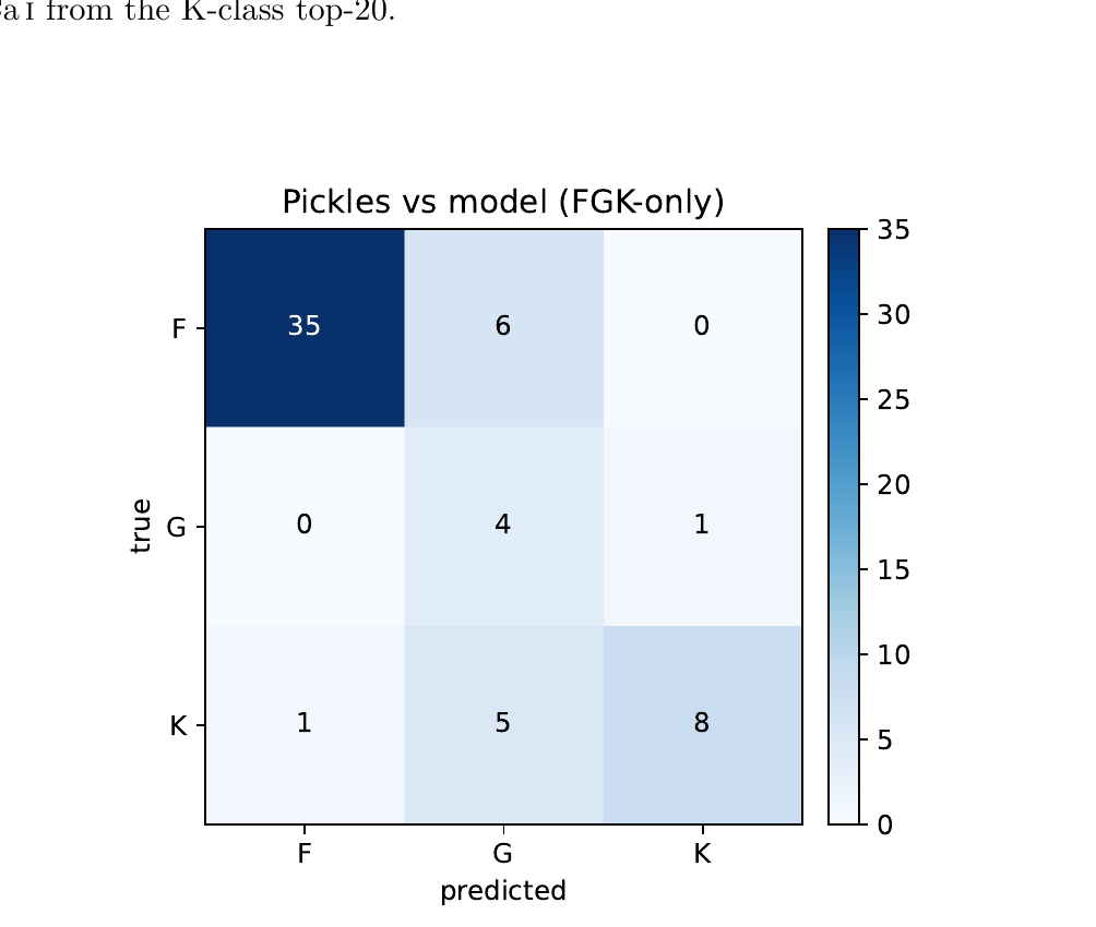
I attempted an external chi-squared cross-check against the Pickles 1998 stellar flux library, hoping for independent corroboration. It did not deliver one, and the honest report is that it is exploratory. Under a 200 Å median-filter continuum, model and templates agreed on 68% of the 69 FGK rows that survived that convention, and the disagreement pattern was loosely consistent with the shortcut reading. But two other continuum conventions produced materially different patterns, and none met the agreement bar I set in advance (at least 0.55 agreement on more than 100 rows). The template cross-check is too sensitive to the continuum convention to stand as independent evidence, so the result rests on the masked-line ablation alone. I am reporting the failed corroboration rather than burying it, because that is the standard the audit is supposed to hold itself to.
What I think this means for the field
Strong aggregate metrics on stellar classifiers are not, on their own, evidence of physics-awareness. The ML interpretability literature has known this since Geirhos et al. 2020 named shortcut learning; what is new here is bringing the interventional probe into stellar spectroscopy specifically, with pre-specification, a proper null distribution, and a falsifiable per-class verdict.
So the concrete recommendation: publish a per-class masked-line ablation table next to the macro-F1, the way this paper does. It costs one extra pass over the held-out set per (line set, class) pair, it needs no retraining, and it converts "the model scores well" into "the model needs these lines to score well," which is the claim a spectroscopic result actually wants to make. A classifier that cannot survive that table is not necessarily wrong, but the reader deserves to know which of its classes are riding a proxy.
Honest limits
The audit covers one classifier (LightGBM), one instrument (FLAMES-UVES), one survey (Gaia-ESO DR5.1), and one diagnostic line list (the canonical MK set). The Gaia-ESO target list concentrates on open clusters and known fields, so spectra are not spatially independent. The leakage-aware cross-validation bounds but does not eliminate this contribution. M-class statistics are too thin in the UVES sample to audit reliably, and the bluer Balmer lines and the Ca II H and K diagnostics fall outside the U580 window. The MK system also encodes luminosity class (dwarf, giant, supergiant) that this paper ignores.
A 3,032-star sample is an order of magnitude smaller than what neighbouring papers (Candebat et al. 2024 on FLAMES-GIRAFFE) work with. The audit instrument generalizes to those larger samples without architectural change because the intervention is defined on the input domain, not on internal model representations.
Why I wrote this paper
I came to this problem by way of a different one. I had a strong-looking classifier and the usual SHAP plots, and I could not bring myself to trust the SHAP plots. They told me which features the model used a lot. They did not tell me which features the model needed. The leap from correlation to intervention is small in the abstract and large in practice: it forces you to write down the prediction before you run the experiment, set the null distribution, and live with the verdict. Two of three pre-specified pairs landed where they were supposed to. The third, Mg b on K, did not, and now I trust the audit.
If you work in stellar machine learning, I would value your views on whether masked-line ablation should become a default reporting standard alongside aggregate metrics, and on what it would take to extend the audit to luminosity class and to the OBA and M ends of the MK sequence.
- Manuscript: completed May 2026; arXiv submission pending.
- Code: github.com/TirtheshJani/ges-uves-mk-audit (MIT)
- Trained model, feature matrix, and numerical artifacts: Zenodo deposit (DOI pending)
- Get in touch: tirtheshjani@gmail.com