A masked-line ablation audit of a LightGBM F/G/K classifier for Gaia-ESO UVES spectra
A LightGBM classifier reaches 0.926 macro-F1 on Gaia-ESO UVES spectra. Masking the diagnostic lines fixed in advance shows which classes depend on which windows, and separates a train-test scale mismatch from a shortcut.
TL;DR. A LightGBM classifier sorts 3,032 Gaia-ESO UVES spectra into three effective-temperature classes, F, G and K, with a held-out macro-F1 of 0.926. For line windows fixed before the test set was scored, I mask each window, rescore the unchanged model and compare the per-class recall change against 5,000 class-matched random windows. Masking the Balmer lines removes almost every F and G prediction (recall drops of 0.840 and 0.917). Masking Mg b lowers G recall by 0.257, in the direction a temperature estimator would move. The K class does not depend on any narrow window: no line set moves more than 3 of 145 K stars, partly because K is 73% giants while F and G are almost all dwarfs. A polynomial re-normalisation of the test spectra collapses G recall from 0.965 to 0.148; a uniform rescaling by 1.09 roughly reproduces the collapse and retraining restores macro-F1 to 0.915, so that collapse is a train-test scale mismatch, not a shortcut. Submitted to RAS Techniques and Instruments, October 2026. Code, model and every number-producing script are public.
New to the astronomy or the statistics? A glossary at the end defines every term used here.
A machine learning model trained on stellar spectra reaches a macro-F1 of 0.926. By every conventional metric, that is a strong classifier. The natural reaction is to ship it, write the paper and move on.
This paper is about what happens when you do not move on. It asks a narrower question than "how well does the model score": when the classifier calls a star F, G or K, does it need the spectral features a spectroscopist would read, and where does the answer depend on choices I made rather than on the star?
The setting in plain terms
Stars are sorted by temperature into spectral classes that run hot to cool: O, B, A, F, G, K, M. The Sun is type G. Astronomers identify class by looking at specific absorption lines in a star's spectrum. Hot and intermediate stars show strong hydrogen Balmer lines (Hα at 6563 Å, Hβ at 4861 Å). Cooler stars show the Mg b triplet near 5170 Å and neutral metal lines such as the Na D doublet at 5890 Å and Ca I at 6162 and 6439 Å. Those are the canonical diagnostics, the lines a working spectroscopist would point at.
One honest caveat up front. The classes in this paper are effective-temperature bins named with MK letters, not spectroscopic MK types. The labels come from the Gaia-ESO parameter catalogue: F is 6000 to 7300 K, G is 5300 to 6000 K, K is 3900 to 5300 K, on a dwarf scale. The bins are applied to giants as well as dwarfs, so luminosity class is a hidden variable. That matters later.
Why a ranking is not a test
The standard tools for opening up a model are permutation importance, SHAP and saliency maps. They rank features by how the model uses them. They do not test whether a feature matters in a falsifiable sense. A bin can rank high because it correlates with a temperature proxy the model also reads elsewhere, and rank low because the model has redundant predictors and treats it as substitutable. Neither outcome tells you what happens if you remove the feature and ask the model to classify again.
So the audit is an intervention on a fixed model. For each (line set, class) pair, the bins inside the window are replaced by a linear interpolation across the gap, the edited spectra are rescored by the unchanged model, and the change in class recall is the readout:
ΔA(L, k) = recall of class k with line set L masked, minus baseline recall of class k.
Each ΔA comes with a 95% bootstrap interval from 2,000 resamples of the test rows, the number of rows that flipped from correct to incorrect (and back), an exact McNemar test on the discordant pairs, and a Monte Carlo p-value against a class-matched null: 5,000 random windows of the same bin count, drawn from regions that avoid every catalogued line, masked the same way. The line sets and the class assignments were logged in a dated decision log on 2026-04-29, before the test set was first scored on 2026-04-30. Logged in version control rather than with an external registry, so "pre-specified", not "pre-registered". The paper carries a deviations-from-plan section that lists what changed after that date and why.
The data and the classifier
The spectra are FLAMES-UVES U580 observations from the Gaia-ESO Survey, taken at the VLT in Chile, covering 4800 to 6800 Å. Labels come from the Gaia-ESO DR5.1 parameter catalogue on the ESO Science Archive. After cross-matching 6,143 catalogue rows to the UVES store and cutting to median signal-to-noise of at least 20 and at most 10% missing bins, 3,032 spectra remain: 536 F, 1,534 G, 962 K. Each spectrum is rebinned by a factor of 5 to 696 log-uniform bins. The 22 bins inside the inter-chip gap (5771 to 5832 Å) are flagged and excluded from the line windows and the null; they are not imputed.
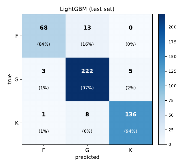
The model is LightGBM, gradient-boosted decision trees, with 500 trees of depth 8 and 63 leaves, balanced class weights and early stopping on a separate validation split (best iteration 120). A fixed 70/15/15 split gives 2,122 training, 454 validation and 456 test spectra. On the test set:
- F: precision 0.944, recall 0.840, F1 0.889 (n = 81)
- G: precision 0.914, recall 0.965, F1 0.939 (n = 230)
- K: precision 0.965, recall 0.938, F1 0.951 (n = 145)
- Macro-F1: 0.926, accuracy 0.934
Recall is quoted to three decimals because per-class recall on the held-out set is the same quantity as the per-class baseline the ablation table is measured against.
Held-out test set · 456 spectra
Gaia-ESO targets concentrate in open clusters and calibration fields, so spectra are not spatially independent and a plain cross-validation can leak field-level structure between folds. Five-fold stratified cross-validation on the train and validation rows gives macro-F1 0.913 (population standard deviation 0.012). Grouping folds by DBSCAN clusters on sky position gives 0.903 (0.016), and grouping by the survey's own field identifier gives 0.906 (0.018). The field-grouped estimate is 0.006 below the plain one, inside the 0.010 fold-to-fold spread, so no field-mate leakage is detectable at the resolution of a single five-fold split. The held-out test split is not group-aware, and the paper says so.
The audit, one pair at a time
Five line sets were masked: the two Balmer lines together (80 Å, 29 bins), Mg b (21 Å, 8 bins), Na D (11 Å, 4 bins), Ca I (8 Å, 2 bins), and a post hoc Fe I and Cr I set built after the SHAP analysis (34 Å, 13 bins). Three pairs were designated headline pairs before scoring: (Balmer, F), (Mg b, G) and (Mg b, K). The gate was that at least two of the three must reject the class-matched null.
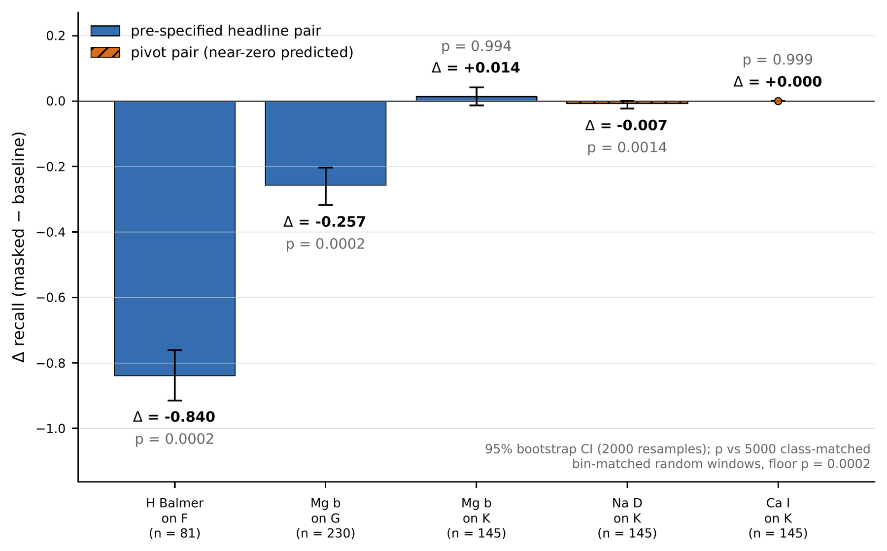
| Line set | Class | ΔA (recall) | 95% CI | Rows lost / gained | Monte Carlo p |
|---|---|---|---|---|---|
| H Balmer | F | -0.840 | [-0.915, -0.761] | 68 / 0 | 0.0002 (floor) |
| H Balmer | G | -0.917 | [-0.952, -0.882] | 211 / 0 | 0.0002 (floor) |
| Mg b | G | -0.257 | [-0.318, -0.203] | 59 / 0 | 0.0002 (floor) |
| Mg b | K | +0.014 | [-0.013, +0.042] | 1 / 3 | 0.994 |
| Na D | K | -0.007 | [-0.023, 0.000] | 1 / 0 | 0.0014 |
| Ca I | K | 0.000 | [0.000, 0.000] | 0 / 0 | 0.999 |
The first three rows are what an astronomer would draw on a napkin. Strip the Balmer windows and the F class has nothing left to stand on; 63 of the 68 lost F rows go straight to K rather than to the adjacent G, which is the signature of an off-manifold input resolving to a default class rather than a graded temperature shift. The paper reports the Balmer result as a firm statement that the model cannot tolerate removal of those windows, and treats the size and direction of the errors as properties of the edit rather than measurements of stellar physics. The Mg b result on G is cleaner: 41 of the 59 lost G rows are read as F and 18 as K, all 59 are dwarfs, and their median temperature sits beside the F/G boundary. Removing a feature that is stronger in cooler stars makes the model answer "hotter", which is what a temperature estimator would do.
The gate passed, two of three. The third headline pair, (Mg b, K), came out at +0.014 with an interval that includes zero. That is the outcome expected under the null, and it is not evidence of anything else.
The K class responds to no narrow window
Across all five line sets, no mask loses more than 3 of 145 K rows. The exact one-sided 95% upper bound on the loss rate is at most 0.053 for any single line set, 0.032 for Mg b and Na D, and 0.020 for Ca I. K recall can even rise: masking the Balmer lines gains 8 K rows, the same "make a star look cooler" response seen on G, running the other way.
A near-zero ΔA with a high Monte Carlo p-value is easy to over-read, so the paper is careful about what it claims. The Monte Carlo p for K says only that the window is unusual among random windows of its width; for K the null distribution is itself concentrated at zero, so one lost row can already look unusual. The K statements therefore rest on flip counts, exact McNemar tests and the Clopper-Pearson upper bounds, not on the p-values. The post hoc Fe I and Cr I set loses 3 K rows and is reported as suggestive at most.
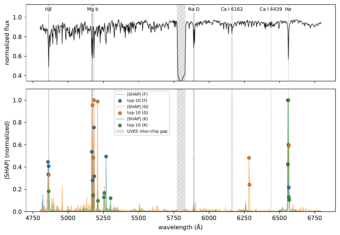
Two further checks pin down what "K does not respond" can mean. First, a positive control: masking all five line sets jointly, or the 20, 50 or 100 bins with the largest validation-set SHAP for K, never lowers K recall under interpolation. Under a constant fill over those 100 bins, K recall drops by 0.166 (25 of 145 rows), so the audit can register a K dependence once enough redundant bins are removed; the K class simply has many temperature-sensitive bins and a narrow mask removes little the others cannot supply. Second, the luminosity confound. In the full sample 97.9% of F rows and 98.2% of G rows are dwarfs (log g above 3.5) and 72.8% of K rows are giants. The test K rows are 107 giants and 38 dwarfs, and the giants lose 0 rows under every narrow mask. K rows also sit far from the class boundaries: median distance 433 K to the nearest bin edge, against 180 K for F and 211 K for G. "K versus G" in this sample is partly "giant versus dwarf", and a feature that tracks temperature in dwarfs is not the feature a tree ensemble needs to separate a giant branch from a dwarf branch.
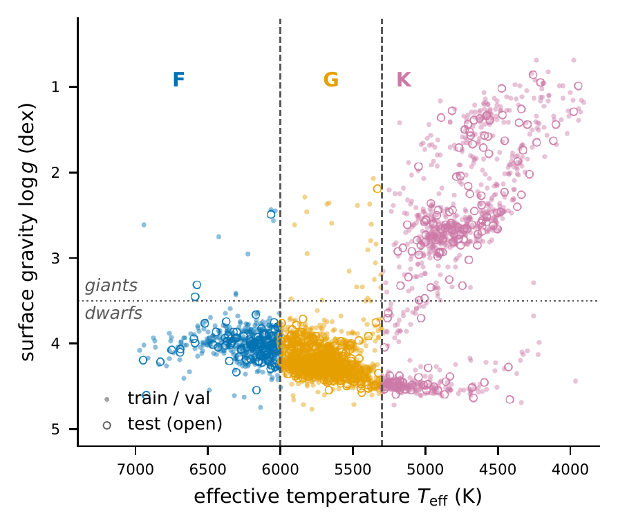
An earlier draft of this work read the K result as a shortcut, with the model substituting Fe I and Cr I lines for the textbook diagnostics. The submitted paper does not make that claim. Under the definition it adopts (a feature predictive in training, outside the pre-specified diagnostic set, whose removal degrades performance under a shift), the Fe I and Cr I result does not qualify, and the luminosity structure is the simpler explanation.
The collapse that was not a shortcut
The largest effect in the paper came from the continuum, and it took the longest to read correctly.
The Gaia-ESO pipeline normalises each spectrum before it reaches the model. Under that normalisation, the per-row median flux outside the chip gap differs by class: 0.929 for F, 0.918 for G, 0.902 for K, a spread of 2.6 points that is monotone with temperature. Re-derive the continuum on the test rows with a sigma-clipped fifth-order Legendre fit instead, and all three medians land just above 1.0 (1.001, 1.003, 1.006), in the reverse order and with a spread of half a point. Score the unchanged model on those re-normalised spectra and G recall falls from 0.965 to 0.148, macro-F1 from 0.926 to 0.475, with 126 of 230 G rows now called K.
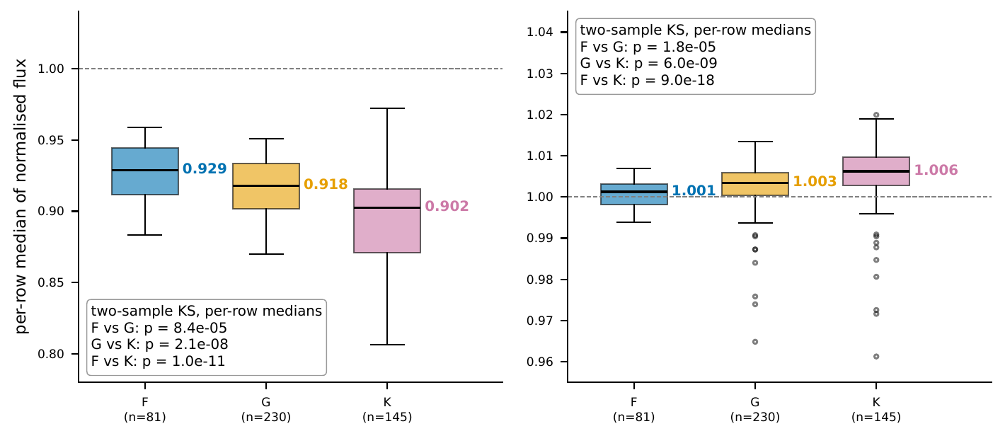
The tempting reading is that the model was using the per-class continuum level as a hidden G-versus-K discriminator. Three experiments say otherwise.
- Remove the spread but keep the scale (rescale every row to the common test median): macro-F1 0.910, 5 G rows go to K. The class-dependent level is not what carries performance.
- Keep the spread but shift the scale (multiply every row by 1.09, the ratio of the polynomial to the production global median): macro-F1 0.550, 127 G rows go to K. A uniform rescaling reproduces the collapse.
- Retrain LightGBM with the same hyperparameters on the polynomial-normalised features: macro-F1 0.915, within the fold-to-fold spread of the production model. The Mg b effect on G survives every retrain (-0.152 to -0.213), and the Mg b effect on K stays null.
Gradient-boosted trees split on absolute thresholds, so a level shift of 9% can move every bin across a split while the labelling rule stays fixed. That is a train-test scale mismatch: a failure to transfer to a normalisation convention the model never saw, not a non-physical feature the model learned. A one-feature logistic regression on the row median reaches only 0.386 accuracy on the test set, so the level carries weak class information, far too weak to explain a G recall of 0.965. The paper reports this as a scale effect and gives the decomposition, and the practical recommendation that follows: anyone scoring a tree model on re-normalised spectra should report the normalisation convention and the global median level, and check sensitivity to a uniform rescaling, before reading any drop as a property of the model.
An external cross-check that did not pass
I compared each test spectrum with the 131 templates of the Pickles (1998) library by chi-squared, and read the spectral type from the template's FITS header. The gate, set on the day of the first run, was agreement of at least 0.55 on at least 100 compared rows. The best result was 0.531 under a 200 Å median-filter continuum, and under that convention 53% of the best-matching templates were supergiants, a luminosity class essentially absent from the sample. The polynomial convention matched no F, G or K template at all. A template library without luminosity or metallicity matching cannot test a three-class temperature classifier at this resolution. The check is reported as failed, in an appendix, rather than dropped.
What the audit adds, and what it does not
A list of windows fixed in advance, a per-class readout and a class-matched null make "does this classifier depend on this window for this class" a reproducible question. The flip counts and the exact McNemar test keep the K-class statement honest about how few rows move. The method works on the input domain of a fixed model, so it needs no retraining and is model-agnostic in principle.
What it does not do: separate a physical dependence from a response to an edited input. Masking and interpolation leave the data manifold, and the Balmer result in particular is a statement about what the model does with an off-manifold spectrum, not a measurement of how much Balmer physics the model encodes. It measures reliance on a window, not the causal effect of a stellar property. The audit covers one classifier, one instrument, one survey and one wavelength setting. M-class statistics are too thin in the UVES sample to audit, and the test split is not group-aware.
Why I wrote this paper
I had a strong-looking classifier and the usual SHAP plots, and I could not bring myself to trust the SHAP plots. They told me which bins the model used a lot. They did not tell me which bins the model needed. Writing the prediction down before running the experiment, setting the null, and living with the verdict turned out to be the useful discipline, and the discipline cut both ways: the same habit that confirmed the Balmer and Mg b results is what forced me to retract the shortcut story I had told myself about the K class and the continuum. Two of three headline pairs landed where they were supposed to. The third did not, and the paper is more honest for it.
If you work on survey spectra and tree models, I would value your views on whether a per-class masked-line table and a uniform-rescale sensitivity check should ship alongside the macro-F1 by default.
Glossary
The astronomy
- Spectrum. The light from a star spread out by wavelength. Dark dips in it are absorption lines, where atoms in the star's atmosphere soak up light at specific wavelengths.
- Ångström (Å). The wavelength unit used here. One ångström is a tenth of a nanometre; this sample covers 4800 to 6800 Å, roughly blue-green to red.
- Spectral class (O, B, A, F, G, K, M). The traditional sequence of star types from hottest to coolest. The Sun is a G star. In this paper F, G and K are temperature ranges, not types read off the spectrum by eye.
- MK system. The Morgan-Keenan scheme that assigns each star a spectral class and a luminosity class (dwarf, giant, supergiant). Only the letters are borrowed here.
- Effective temperature. The surface temperature a star would have if it radiated as a perfect blackbody. The class labels are bins of it: F is 6000 to 7300 K, G is 5300 to 6000 K, K is 3900 to 5300 K.
- Dwarf and giant. A dwarf is a star in the long, stable middle of its life, like the Sun. A giant has exhausted the hydrogen in its core and swollen. At the same temperature the two have different spectra.
- Surface gravity (log g). How strongly a star pulls at its surface, on a log scale. Giants are puffed up, so their gravity is low. This paper counts log g above 3.5 as a dwarf.
- Kiel diagram. A plot of surface gravity against effective temperature. Dwarfs and giants fall on separate branches.
- Balmer lines. Absorption lines of hydrogen. Two fall in this range: Hα at 6563 Å and Hβ at 4861 Å. They are strongest in A and F stars and fade as stars get cooler.
- Mg b triplet. Three magnesium lines near 5170 Å that grow stronger in cooler stars. A standard temperature and gravity indicator for G and K stars.
- Na D doublet. Two sodium lines near 5890 Å, strong in cool stars.
- Ca I and Fe I, Cr I. Lines of neutral calcium (6162 and 6439 Å), iron and chromium. The roman numeral I means the atom still has all its electrons.
- Continuum and normalisation. The continuum is the smooth background a spectrum would have without any lines. Normalising divides it out so that the continuum sits at 1.0 and lines show as dips below it. Two reasonable ways of estimating the continuum can leave the whole spectrum at slightly different levels.
- Gaia-ESO Survey. A large public spectroscopic survey of about 100,000 stars in the Milky Way, run on the European Southern Observatory's Very Large Telescope in Chile.
- FLAMES-UVES. The high-resolution spectrograph that took these spectra. U580 is the instrument setting, centred at 580 nm.
- Inter-chip gap. A stretch of wavelengths (5771 to 5832 Å) that falls between the instrument's two detectors and has no data.
- Pickles library. A published set of 131 reference spectra, one per stellar type, used here as an outside check.
The model and the scores
- LightGBM. A gradient-boosted decision-tree library. The model is many small trees, each correcting the last, and each tree splits on thresholds such as "flux in this bin below 0.82".
- Bin. One wavelength slot in the input. Each spectrum is rebinned to 696 bins, and each bin is one feature for the model.
- Training, validation and test split. The data is cut into three parts: one to fit the model, one to tune it, and one held back and scored once. All headline numbers come from the 456 test spectra.
- Precision. Of the stars the model called G, the share that really are G.
- Recall. Of the stars that really are G, the share the model called G. The audit reads its results as changes in recall.
- F1 and macro-F1. F1 combines precision and recall for one class into a single score between 0 and 1. Macro-F1 is the plain average of F1 across the three classes, so a small class counts as much as a large one.
- Confusion matrix. A table of true class against predicted class. Correct calls sit on the diagonal.
- Cross-validation. Re-splitting the training data several ways and averaging the scores, to see how much a result depends on one particular split. Grouped cross-validation keeps stars from the same sky field together so that near-duplicates cannot leak between folds.
- Permutation importance and SHAP. Two ways to rank which inputs a model leans on. Permutation importance shuffles one input and measures the loss; SHAP splits each prediction into contributions from each input. Both rank. Neither tests what happens when the input is removed.
The audit
- Ablation. Removing part of the input and measuring what changes. Here a line window is cut out of every test spectrum and the gap is bridged with a straight line (interpolation).
- ΔA. The change in a class's recall when a line set is masked. A ΔA of -0.840 means the model now gets 84 percentage points fewer of that class right.
- Line set and window. A line set is a group of absorption lines tested together; its window is the wavelength range masked.
- Pre-specified. The line sets, the classes they were expected to affect and the pass mark were written down, dated, before the test set was first scored. "Pre-registered" would imply an outside registry, which was not used.
- Headline pair and gate. Three (line set, class) pairs were picked in advance as the main tests. The gate was that at least two of the three had to show a real effect.
- Null and class-matched random windows. The null is what you expect if a line does not matter. To build it, 5,000 random windows of the same width, placed away from any known line, are masked the same way. A real line effect has to beat almost all of them.
- Monte Carlo p-value. The share of those random windows that did at least as much damage as the real one. With 5,000 draws the smallest possible value is 0.0002, the "floor" in the table.
- Bootstrap confidence interval. A range for ΔA found by resampling the test stars with replacement 2,000 times and recomputing. A 95% interval that excludes zero means the effect is unlikely to be noise from which stars happened to be in the test set.
- Flip counts and McNemar test. Flip counts are how many stars went from right to wrong, and wrong to right, when a window was masked. McNemar's test asks whether those two counts are too lopsided to be chance.
- Clopper-Pearson upper bound. An exact upper limit on a rate when very few events are seen. Losing 0 to 3 of 145 K stars puts the true loss rate at no more than about 5%.
- Positive control. A test built to make sure the method can detect an effect when one should exist, here masking the bins the model ranks highest for K.
- Off-manifold input. An input unlike anything the model saw in training. A spectrum with its Balmer lines cut out is one, so the model's answer to it says more about the edit than about stellar physics.
- Shortcut. A feature that predicts the label in training but is not the property you meant to measure, so the model breaks when conditions shift. The paper tests for one and does not find one.
- Train-test scale mismatch. The model was trained on spectra at one overall level and tested on spectra at another. Tree splits sit at fixed thresholds, so a uniform 9% shift moves stars across them even though nothing about the stars changed.
- Manuscript: submitted to RAS Techniques and Instruments, October 2026. arXiv submission pending.
- Code: github.com/TirtheshJani/ges-uves-mk-audit (MIT), with the dated decision log and every number-producing script.
- Trained model, feature matrix and numerical artifacts: Zenodo, v1.2.0
- Get in touch: tirtheshjani@gmail.com