Will I Hit My Target? A Monte Carlo Planner with ML Inputs

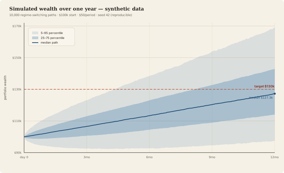
Here is a question with a real answer. I start with $100,000, I add $50 at the end of every trading day, and I want $130,000 in a year. What are the odds I get there? I built a Monte Carlo planner to answer exactly that, and on the synthetic dataset it comes back with 45 percent. The median outcome lands at $127,300, a little short of the $130,000 line. But the number is not the interesting part. What feeds the simulation is.

First the disclaimer, because it changes how you should read everything below. This is a technical and educational project, not financial advice, and it is not validated for real investing. The default configuration runs on a seeded synthetic dataset, four invented tickers called AAA through DDD, so every figure here describes what the tool computes on made-up data, not a forecast of any real market. I will label the numbers as synthetic each time they matter, because they are.

The shape of the pipeline

The pipeline is short to state. Take prices, historical or synthetic. Estimate the inputs a simulation needs: expected returns, volatilities, correlations, and how markets switch between calm and turbulent. Optimize an allocation from those inputs. Simulate ten thousand possible futures of that allocation. Then read the planning answer off the distribution of where they end up.

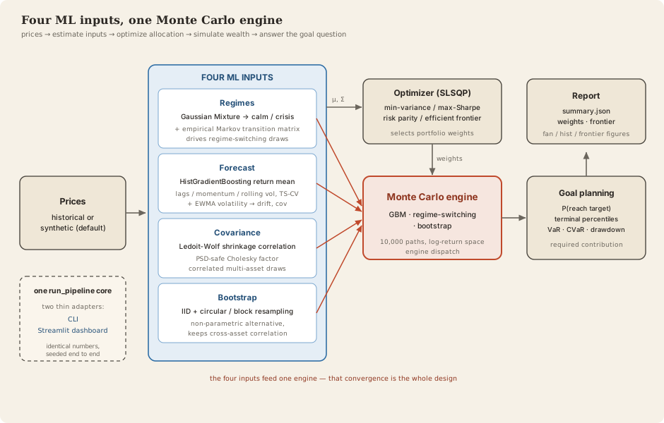
The estimate-the-inputs step is where the machine learning lives, and it is the reason the project exists. Four separate models feed the one engine, each earning its place for a specific reason rather than because it sounded advanced.

Four models, one engine

Regimes. Markets do not have one personality. They have calm stretches and violent ones, and a model that draws every day from a single distribution will understate how bad a bad year can get. So the planner clusters daily returns with a Gaussian Mixture into two regimes, calm and crisis, and estimates a first-order Markov transition matrix empirically: the probability of staying calm, of tipping into crisis, of recovering. On the synthetic run the chain spends about 85 percent of its stationary time in the calm regime and 15 percent in crisis. The regime-switching simulation then walks that chain day by day and draws returns conditional on where it is, so a crisis clusters into a run of bad days the way real drawdowns do, instead of sprinkling single bad days at random.

Forecast. The drift of the simulation, the average return it walks toward, should not just be the historical mean. The planner forecasts the next period's log-return with a HistGradientBoostingRegressor built on engineered features: lagged returns at 1, 5, and 21 days, momentum over 21 and 63 days, and rolling volatility. It scores that model with time-series cross-validation, the kind that only ever trains on the past and tests on the future, because shuffling a time series is how you fool yourself into a great backtest that means nothing. A separate EWMA estimate handles volatility. Together they set the drift and the scale the engine uses.

Covariance. Four assets have six pairwise correlations, and the sample estimate of them from a finite history is noisy enough to wreck an optimizer, which will happily pile into whatever pair looks spuriously diversifying. Ledoit-Wolf shrinkage pulls the noisy sample correlation matrix toward a structured target, trading a little bias for a lot less variance. The planner then takes a PSD-safe Cholesky factor of the result, which is the step that lets it draw correlated returns for all four assets at once without the factorization failing on a matrix that is not quite positive definite.

Bootstrap. Every model above assumes a shape for returns. The bootstrap assumes none. It resamples actual historical return rows, either independently or in blocks that keep short runs intact, and because it resamples whole rows it preserves the cross-asset correlation structure for free. It is the non-parametric check on the parametric machinery: if the fitted models and the resampled history disagree badly, that is a signal worth chasing, not a rounding error.

Choosing the allocation

With the inputs estimated, the allocation is a constrained optimization. The planner offers minimum-variance, maximum-Sharpe, risk parity, and the full efficient frontier, all solved with SLSQP under long-only, fully-invested constraints. On the synthetic run, maximizing the Sharpe ratio put 78.5 percent into CCC and 21.5 percent into AAA, and zeroed BBB and DDD entirely, for a portfolio with a 16.9 percent annualized return, 18.5 percent annualized volatility, and a Sharpe of 0.91. Those are properties of four synthetic assets, so the specific split says nothing about real markets. What it demonstrates is the optimizer doing its job, concentrating in the two assets whose risk-adjusted return and correlation structure it prefers and declining the other two.

The planning answer

Now the question the whole thing was built for. Simulate ten thousand year-long futures of that allocation, add the $50 daily contribution along the way, and read the answer off the distribution of final wealth.

On the synthetic dataset, the plan reaches its $130,000 target in 45.0 percent of the ten thousand paths. The median terminal wealth is $127,300, which is why the odds sit just under half: the middle outcome falls about $2,700 short of the line. The spread is wide. The 5th percentile ends at $97,300, below where it started, and the 95th at $169,000.

The downside has its own summary. Among the paths that miss, the average shortfall is about $16,300. The one-day 90 percent Value at Risk is 1.2 percent, meaning one trading day in ten is worse than a 1.2 percent loss, and the conditional VaR, the average loss on those worst days, is 1.9 percent. The median path's deepest peak-to-trough drop over the year is 11.3 percent. Every one of those is a number about synthetic data, and every one is the kind of number a planner actually needs, because how much you might lose along the way matters as much as where you probably end up.

The most useful output is the inverse question. If a 45 percent chance is not good enough, and for a target this close to the starting point it should not be, how much more do I need to contribute? The planner solves for the contribution that reaches the target at 90 percent confidence, and the answer on the synthetic run is about $163 per period against the $50 I started with. Having to more than triple the deposit to move from a 45 percent chance to a 90 percent one is exactly the kind of concrete, unglamorous tradeoff the tool exists to surface.

One core, two interfaces

Two things about how it is built are worth stating, because they are what make the numbers above trustworthy.

The first is that there is one core. A single run_pipeline function does the estimate-optimize-simulate-plan sequence, and both the command-line tool and the Streamlit dashboard are thin adapters over it. They cannot drift apart, because they run the same code and report the same numbers for the same config. The second is that the whole thing is seeded end to end: numpy's generator for the sampling, and a fixed random_state on every scikit-learn estimator. Run it twice and the output is identical, which I check with a reproducibility test rather than trust. That is what lets me quote a $127,300 median and mean it: the run behind this post reproduces bit for bit from the config and the seed. The suite around it is 89 test functions across 18 files, one module per core module plus the reproducibility and CLI checks, and it all runs offline on the synthetic data.

The design calls I would defend

A few decisions went the less obvious way, and they are the ones I would defend in a review.

The simulation runs in log-return space, because log returns compound by addition and that is what a Monte Carlo step wants. But portfolio returns do not aggregate correctly in log space; a weighted sum of log returns is not the log return of the weighted portfolio. So the engine converts to simple returns to combine the assets at each step, then back to log space to compound forward. It is a small conversion that is easy to skip and quietly wrong if you do.

The contribution is applied once per simulation period, and the default period is one day. A $50 contribution therefore means roughly $12,600 a year, not $50 a month. That is a modeling choice worth saying out loud rather than burying, because it is exactly the sort of unit mismatch that makes a planner's output look inexplicable until you find it.

And there is no hidden Markov model. A full HMM would couple the regime inference and the transition estimation into one harder fit. The planner instead clusters with a Gaussian Mixture and estimates the transition matrix empirically from the resulting labels. It gives regime-switching dynamics with one well-understood dependency and no bespoke inference loop to debug, a deliberate trade of a little statistical elegance for a lot of maintainability.

What it is not

The limitations are the honest part, so they go last and unhedged. The default data is synthetic, four invented tickers, which is what makes the project reproducible from a clean clone with no accounts, and also what makes every number here a demonstration rather than a prediction. There is a yfinance path for real market data, but I have put no live-performance claim behind it, and this post makes none. The gradient-boosting forecaster is a component that sets the drift, not an oracle; nothing here says it predicts real returns well, because I have not tested that and it is not what the project is for. A Monte Carlo planner is only ever as good as its return model, so a 45 percent probability on synthetic data is a statement about the model's assumptions, not a fact about anyone's future.

What it is, is a working pipeline where four machine-learning models each feed a simulation for a reason you can point to, wired into one reproducible core that answers a question people actually ask. The code is on GitHub, synthetic config and tests included, if you want to run it and get the same numbers.

Code: https://github.com/TirtheshJani/Monte-Carlo-Simulations