In this blog post, I’ll take you through my project journey, where I embarked on building a neural network from scratch using only NumPy. This endeavor was not just a programming exercise but a deep dive into the underpinnings of machine learning models. Whether you’re a seasoned coder or new to the tech world, I hope my experiences and insights can shed some light on the fascinating world of neural networks.
The Genesis
The first step was to import the necessary Python libraries: NumPy for numerical computations, Pandas for data manipulation, and Matplotlib for visualizing the data. These tools are staples in the data science toolkit, providing a robust foundation for handling and analyzing complex datasets.
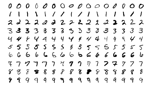
My dataset resided in a CSV file, containing pixel values of handwritten digits along with their corresponding labels—a perfect dataset for a classification task. Using Pandas, I loaded the data and took a peek at the first few rows with df.head(). Each row represented an image of a handwritten digit, with the first column being the label (the digit) and the following 784 columns (28×28 pixels) the pixel values.
Preprocessing
The raw data needed to be converted into a format suitable for the neural network. I transformed the Data Frame into a NumPy array to leverage NumPy’s powerful numerical operations. Recognizing the potential for overfitting, I partitioned the data into training and cross-validation sets. This split would later help in tuning the model’s parameters to improve its generalization capabilities.
The Neural Network
The core of my project was the implementation of a simple yet effective neural network. The network consisted of two layers: a hidden layer and an output layer, each with its weights and biases. The initialization of these parameters was random, adhering to the principle that starting points matter in the journey of optimization.
Activation Functions: Bringing Non-linearity
To introduce non-linearity, I used the Rectified Linear Unit (ReLU) function for the hidden layer and the softmax function for the output layer. These choices are common in neural network architectures due to their computational efficiency and effectiveness in model training.
Forward Propagation: A Leap of Faith
The forward propagation process involved calculating the linear transformations and activations for both layers. This step was crucial for generating predictions from the input data.
Backward Propagation: Learning from Mistakes
Learning in neural networks occurs through backward propagation. By comparing the predictions with the actual labels, I computed gradients for the weights and biases. This information directed how to adjust the parameters to reduce the error in predictions.
Iterative Optimization
The training process was iterative, employing gradient descent to update the parameters in small steps. Each iteration brought the model closer to its goal—minimizing the loss function and improving its accuracy on the training data.
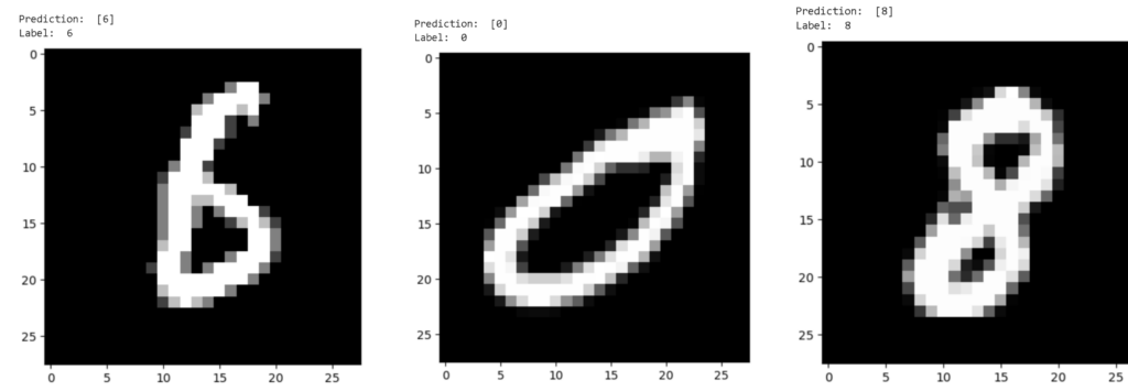
Results
After numerous iterations, the model’s performance on unseen data (the cross-validation set) was promising. This success was a testament to the power of simple neural network architectures when armed with the right techniques and a systematic approach.
This project was a profound learning experience, demystifying the workings of neural networks and reinforcing the importance of foundational principles in machine learning. It’s a journey that has just begun, with endless possibilities and challenges ahead.
I hope this account of my project has illuminated some aspects of neural networks and inspired you to embark on your own projects. The blend of theory and practice in machine learning is a powerful tool for solving complex problems, and it’s within reach for anyone willing to learn and explore.
Check out more projects on my Github profile: https://github.com/TirtheshJani/NN-with-math-and-numpy
